Advantages of Rotary Direct Drives
Increases Dynamic Capacity
- No conversion of motion form
- The drive train is free of elasticity, backlash, hysteresis and has few friction caused by transmission or coupling elements.
- Multi-pole motor
- With a multi-pole design, IDAM motors are capable of producing very high torque. In addition, this high torque can be used from rotary speed > 0 right up to the continuous speed.
- Thin, ring-shaped rotor
- Thanks to the thin, ring-shaped design with a large, open inner diameter, the motor has a very low rotor inertia. This allows for very high motor acceleration capabilities.
- Direct measurement of position
- Thanks to direct position measurement and the rigid mechanical structure, positioning is performed dynamically and highly accurate.
Reduces Operating Costs
- No additional moving parts
- Assembly, adjustment and maintenance work for the drive assembly is reduced.
- No wear in the drive train
- Even under high and frequently alternating loads the drive train is extremely durable. Machine downtimes drop as a result.
- High availability
- In addition to increased service life and reduced wear, the robustness of the torque motors increases the system availability.
Increases Design Flexibility
- Hollow shaft
- With its large, open, inner diameter, the hollow shaft design of a torque motor allows for much greater design flexibility. The hollow shaft allows for tubing, fixtures, rotary unions and wiring to travel up through the center of the motor.
- Component integration RDDS
- Thanks to the smaller space required, the system can be easily integrated into the machine design.
- Compact design
- Along with the large, open inner diameter (hollow shaft), systems are very compact relative to the torque output.
- Low number of components
- The mature design facilitates the integration of the system in the overall machine concept. Fewer and more robust parts result in a low failure rate (high MTBF*).
*MTBF: Mean Time Between Failures
System Advantages
- High dynamics and stiffness
- Extremely smooth motion
- High acceleration
- High velocity
- Compact design
- Easy assembly
- Excellent static and dynamic load rigidity
- No backlash
- Low-wear and low-maintenance system
- Small inertia
- Peak torque Tp: 8.9 – 369 Nm
- Measuring system: Optical measuring principle, several increments depending on model
- Bearing: Compact, high external tilting torque, high stiffness and accuracy, very low axial and radial runout
- Free inner diameter
Standard Design
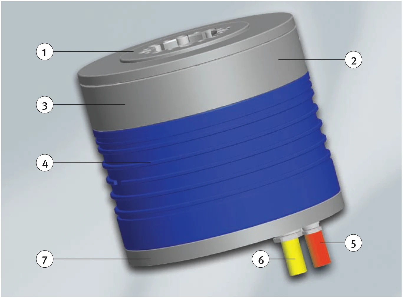
RDDS Standard Design: component 1 (stage plate) to 7 (base plate) position diagram
The RDDS standard design comprises the following seven components:
Thermal Motor Protection
Monitoring Circuit I and II
Direct drives are often being operated at their thermal performance limits. In addition, unforeseen overloads can occur during operation which result in an additional current load in excess of the permissible nominal current. For this reason, the servo controllers for motors should generally have an overload protection in order to control the motor current. Here, the effective value (root mean square) of the motor current must only be allowed to exceed the permissible nominal current of the motor for a short time. This type of indirect temperature monitoring is very quick and reliable.
IDAM motors are equipped with temperature sensors (PTC and KTY) which should be used for thermal motor protection.
Monitoring Circuit I
The three phase-windings are equipped with three series-connected PTCs to ensure motor protection. A PTC is a positive temperature coefficient thermistor. Its thermal time constant when installed is below 5 s.
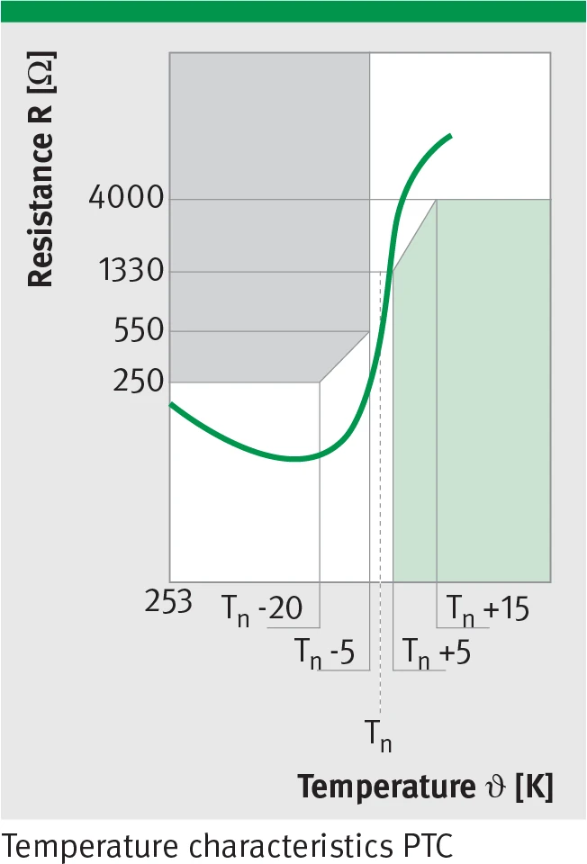
Temperature characteristics PTC: resistance R [Ω] vs. temperature ϑ [K]; resistance rises sharply above nominal response temperature Tn
Temperature Characteristics PTC
Resistance R [Ω] vs. temperature ϑ [K] (extracted from source):
| Temperature | Tn-20 | Tn-5 | Tn | Tn+5 | Tn+15 |
|---|---|---|---|---|---|
| Resistance R [Ω] | 250 | 550 | 1330 | 4000 | — |
Tn: Nominal response temperature
In contrast to a KTY, its resistance increases very sharply when the nominal response temperature Tn is exceeded, increasing to many times the cold value in the process. With three PTC elements connected in series, this behaviour also generates a clear change in the overall resistance even if only one of the elements exceeds the nominal response temperature Tn. The use of three sensors ensures that, even if the motor is at a standstill under an asymmetric phase load, there is a signal for a safe shut-down.
A commercially available motor protection tripping device which is connected downstream will typically trigger between 1.5 and 3.5 kΩ. In this way, overtemperature is detected to within a discrepancy of a few degrees for every winding. The tripping devices also react if the resistance is too low in the PTC circuit, which usually indicates a defect in the monitoring circuit. It also ensures secure electrical separation between the controller and the sensors in the motor. The motor protection tripping devices are not included in the scope of supply.
Note: PTCs are not suitable for temperature measurements. The KTY should be used here if required. Further monitoring sensors can be integrated at the customer's request. As a rule, PTC sensor signals must be monitored for protection against overtemperature.
Monitoring Circuit II
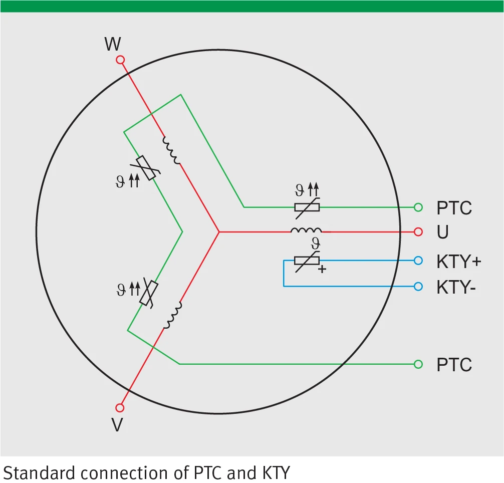
Standard connection of PTC and KTY: three phase-windings (U, V, W) each fitted with PTC; one phase (U) fitted with KTY84-130
On one phase of the motor there is an additional KTY84-130. This sensor is a semiconductor resistor with a positive temperature coefficient.
A temperature-equivalent signal is generated with a delay which depends on the motor type. In order to protect the motor against overtemperature, a shut-off limit is defined in the controller. When the motor is at a standstill, constant currents flow through the windings, with the current depending on the respective pole position.
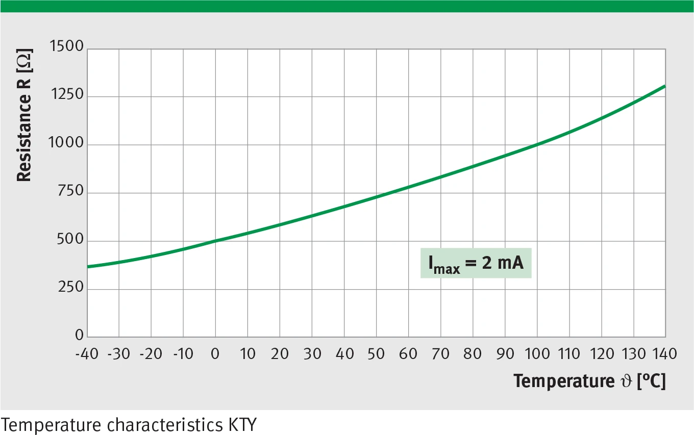
Temperature characteristics KTY: resistance R [Ω] vs. temperature ϑ [°C] (−40 to 140 °C), measuring current Imax = 2 mA
As a result, the motor does not heat up uniformly, which may cause overheating of non-monitored windings. The PTC and KTY sensors have a basic insulation to the motor. They are not suitable for direct connection to PELV/SELV circuits according to standard DIN EN 50178.
Note: The KTY sensor monitors a single winding. Its signal can be used to monitor the temperature or issue a warning. Exclusive use for switching off is not permissible.
Electrical Connections
The standard cable connections of the RDDS1 matrix are axial. Their position is defined in the drawings. The cable length from the motor output is 1.0 m. The wire ends are open and fitted with end sleeves. The cables which are used are UL approved and suitable for cable drag chains.
Optionally the rotary systems are available with externally mounted plug direct on the casing or with coupler plug on the connecting cables.
Positive Direction of Rotation of the System
The standard direction of rotation of the stage plate is counter-clockwise, but it can vary depending on connecting type.
Pin Layout — Cable Connection (Standard)
Type of cable: 4G1.5 + 2x (2x0.75) KAWEFLEX 5281, Ø 12.6 mm, bending radius dynamically 95 mm, bending radius statically 63 mm
| Motor | |
|---|---|
| Core | Signal |
| 1 | Phase U |
| 2 | Phase V |
| 3 | Phase W |
| GNYE | PE |
| 5 | PTC (3x series, all phases) |
| 6 | PTC (3x series, all phases) |
| 7 | + Temperature sensor KTY84-130 (one phase) |
| 8 | - Temperature sensor KTY84-130 (one phase) |
| Shield | |
Type of cable: 12x0.08 NJ AWM STYLE 20963, Ø 3.7 mm, bending radius dynamically 40 mm, bending radius statically 8 mm
| Measuring system 1 Vpp | |
|---|---|
| Core | Signal |
| GN | U1+ |
| BN | U1- |
| BK | U2+ |
| RD | U2- |
| GY | U0+ |
| PK | U0- |
| WH | GND |
| BU | +5 V |
| Shield | |
Pin Layout — Plug Connection (Option)
RDDS1-130xH: 9-pole M17 Mounted Plug
| Motor — 9-pole M17 mounted plug | |
|---|---|
| Pin | Signal |
| 1 | Phase U |
| 2 | Phase V |
| 3 | Phase W |
| PE | PE |
| A | PTC (3x series, all phases) |
| B | PTC (3x series, all phases) |
| C | NC |
| D | + Temperature sensor KTY84-130 (one phase) |
| E | - Temperature sensor KTY84-130 (one phase) |
| Case | Shield |
| Measuring system 1 Vpp — 17-pole M17 mounted plug | |
|---|---|
| Pin | Signal |
| 1 | +5 V Sense |
| 2 | NC |
| 3 | NC |
| 4 | GND Sense |
| 5 | NC |
| 6 | NC |
| 7 | +5 V |
| 8 | NC |
| 9 | NC |
| 10 | GND |
| 11 | NC |
| 12 | U2+ |
| 13 | U2- |
| 14 | U0+ |
| 15 | U1+ |
| 16 | U1- |
| 17 | U0- |
| Case | Shield |
RDDS1-160xH, RDDS1-180xH, RDDS1-230xH and Connecting Variants MA/MU/MD (All Sizes)
RDDS1-160xH, RDDS1-180xH, RDDS1-230xH use an 8-pole M23 mounted plug; connecting variants MA/MU/MD (all sizes) use an 8-pole M23 coupler plug at the cable.
| Motor — 8-pole M23 mounted plug | |
|---|---|
| Pin | Signal |
| 1 | Phase U |
| 4 | Phase V |
| 3 | Phase W |
| 2 / PE | PE |
| A | PTC (3x series, all phases) |
| B | PTC (3x series, all phases) |
| C | + Temperature sensor KTY84-130 (one phase) |
| D | - Temperature sensor KTY84-130 (one phase) |
| Case | Shield |
| Measuring system 1 Vpp — 12-pole M23 mounted plug / coupler plug | |
|---|---|
| Pin | Signal |
| 1 | U2- |
| 2 | +5 V Sense |
| 3 | U0+ |
| 4 | U0- |
| 5 | U1+ |
| 6 | U1- |
| 7 | NC |
| 8 | U2+ |
| 9 | NC |
| 10 | GND |
| 11 | GND Sense |
| 12 | +5 V |
| Case | Shield |
Commutation
Rotary direct drive systems are preferably run in commutated operation. As standard, IDAM torque motors are not equipped with Hall sensors. IDAM recommends measuring system-related commutation, because it is supported by modern servo-inverters and controllers.
Insulation Strength
Insulation strength for link voltages of up to 600 VDC.
IDAM motors comply with EC directive 73/23/EEC and European standards EN 50178 and EN 60204. Prior to delivery they are tested with differentiated high voltage testing methods and casted under vacuum. Please make sure that the type-related operating voltages of the motors are observed.
Overvoltages at Motor Terminals in Converter Operation
Due to the extremely fast-switching power semiconductors which generate high du/dt loads, significantly higher voltage peaks than the actual converter voltages may occur at the motor terminals, particularly when longer connecting cables (from a length of approx. 5 m) are used between motor and converter. This places a very high load on the motor insulation.
Note:
- The du/dt values of the PWM modules must not exceed 8 kV/µs.
- The motor connecting cables must be kept as short as possible.
- In order to protect the motors, an oscilloscope should always be used in the specific configuration to measure the voltage (PWM) applied to the motor via the winding and in relation to PE. The present voltage peaks should not significantly exceed 1 kV. From approx. 2 kV a gradual damaging of the insulation should be expected.
- Please observe the recommendations and configuration notes provided by the manufacturer of the controller.
IDAM engineers will assist you with your application and help you to determine and reduce excessive voltages.
Cooling and Cooling Circuit
Power Loss and Thermal Loss
In addition to the power loss defined by the motor constant km, motors are also subject to frequency-dependent losses occurring especially at higher control frequencies (above 50 Hz). These losses jointly cause the motor and other system assemblies to heat up.
The following rule applies at low control frequencies (< 80 Hz) of the motors: Motors with a high motor constant km produce lower power losses in relation to comparable motors with a lower motor constant.
The power loss generated during motor operation is transmitted via the motor assembly to attached components. The overall system is carefully designed to control the way in which this heat distribution is influenced and controlled through convection, conduction and radiation.
The continuous torques of liquid-cooled motors are around twice as high as those of uncooled motors. The rotary direct drive systems must be selected and integrated into the machine concept in accordance with the requirements for installation space, accuracy and cooling.
Active cooling should be preferably used on machines with high performance and on equipment with highly dynamic operation and correspondingly high bearing loads.
Cooling Design
The cooling of the systems is designed as jacket cooling and should be connected by the customer to the cooling circuit of a cooling device. The cooling jacket is optionally supplied as a part of the motor or is already an integral part of the machine construction for the customer.
The cooling medium passes from the inlet to the outlet through holes in the cooling fins at different levels. Inlet and outlet connections can be assigned to the two connections as required. The flow area is sealed to the outside with O-rings.
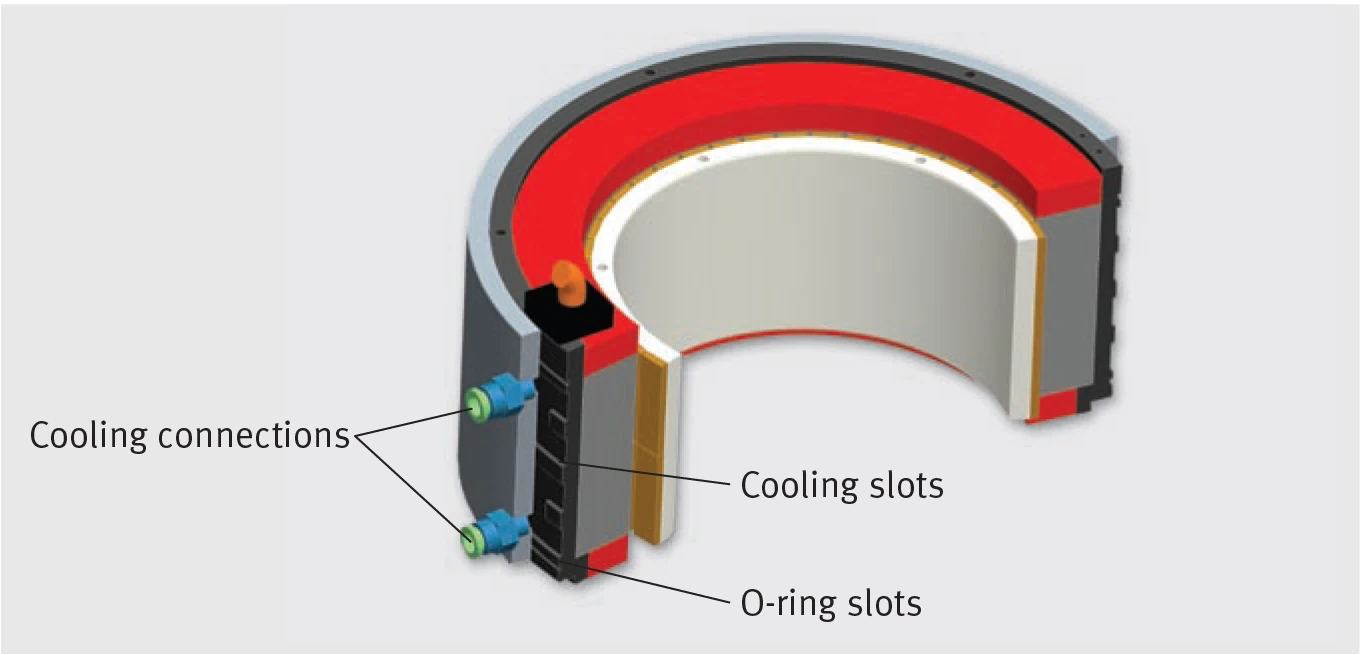
Cooling jacket cross-section: cooling connections, cooling slots and O-ring slots positions
Note: When using water as the coolant, additives must be used which prevent corrosion and biological deposits in the cooling circuit.
Dependency of Characteristic Data on the Supply Temperature of Cooling Medium
The continuous current Icw indicated in the data sheet for water cooled operation can be achieved at a rated supply temperature ϑnV = 25 °C. Higher supply temperatures ϑV result in a reduction of the cooling performance and therefore also the nominal current. The reduced continuous current Ic red can be calculated from the following quadratic equation:
Ic red = Icw × √ϑmax − ϑVϑmax − ϑnV
| Symbol | Description | Unit |
|---|---|---|
| Ic red | Reduced continuous current | A |
| Icw | Continuous current, cooled at ϑnV | A |
| ϑV | Current supply temperature | °C |
| ϑnV | Rated supply temperature | °C |
| ϑmax | Maximum permissible winding temperature (applies to a constant motor current) | °C |
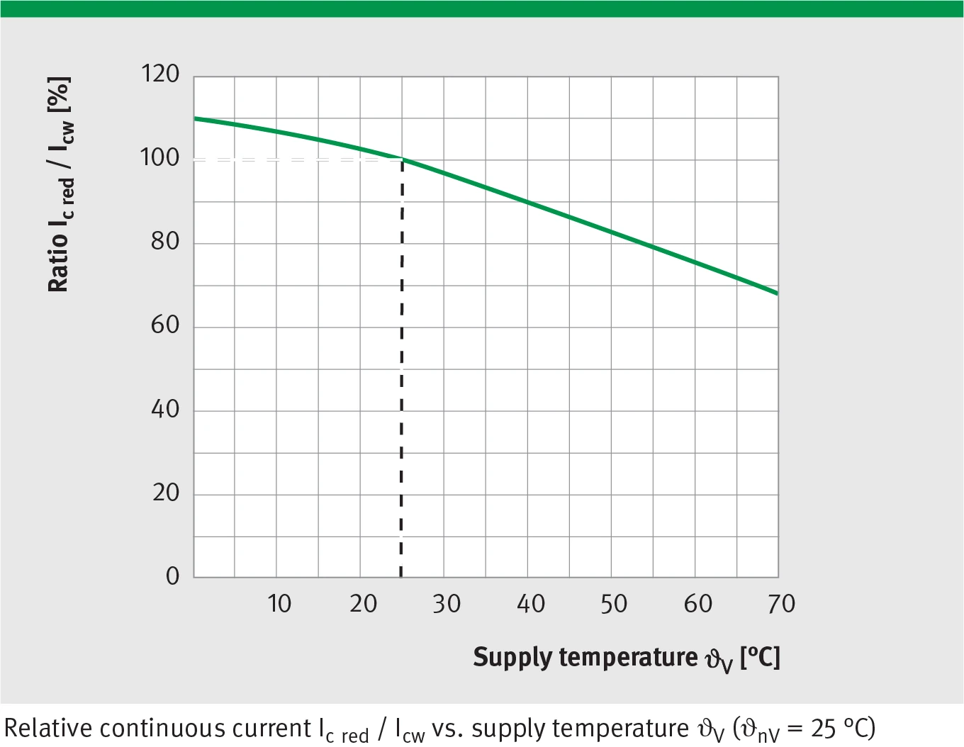
Relative continuous current Ic red / Icw [%] vs. supply temperature ϑV [°C] (rated supply temperature ϑnV = 25 °C)
Positioning Cycle
The following positioning cycle example uses the system RDDS1-160x195-S-B-CA-WM-9000:
Example System Parameters
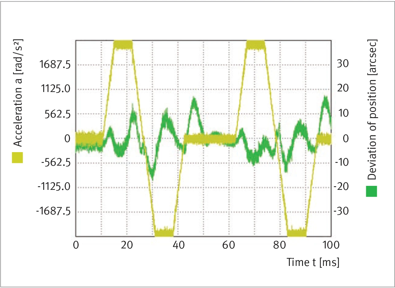
Positioning cycle (left): angular acceleration a [rad/s²] and position deviation [arcsec] vs. time t [ms]
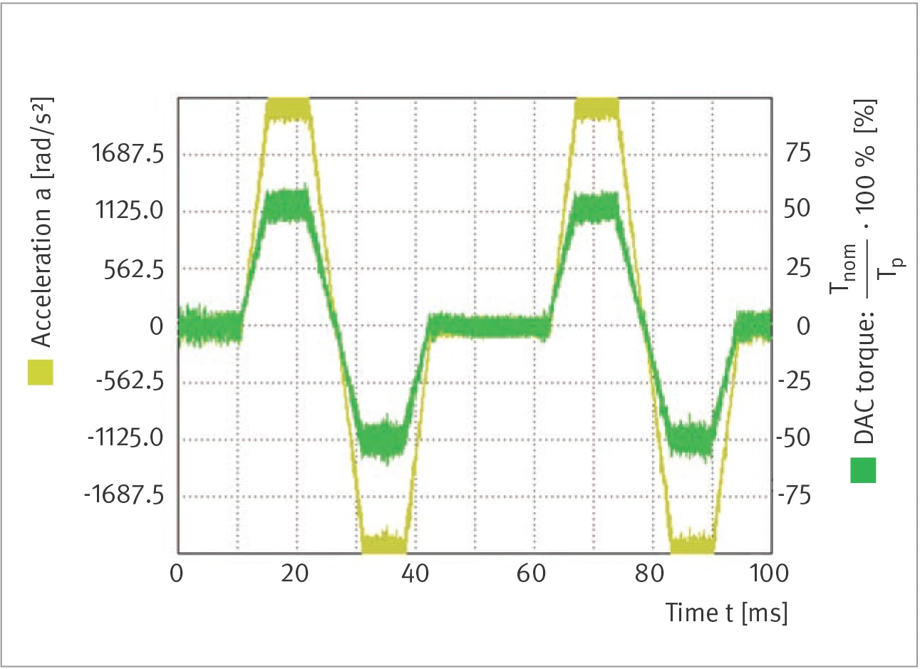
Positioning cycle (right): angular acceleration a [rad/s²] and DAC torque [% Tnom/Tp] vs. time t [ms]
Tp: Peak torque; Tnom: Nominal torque
System Configuration
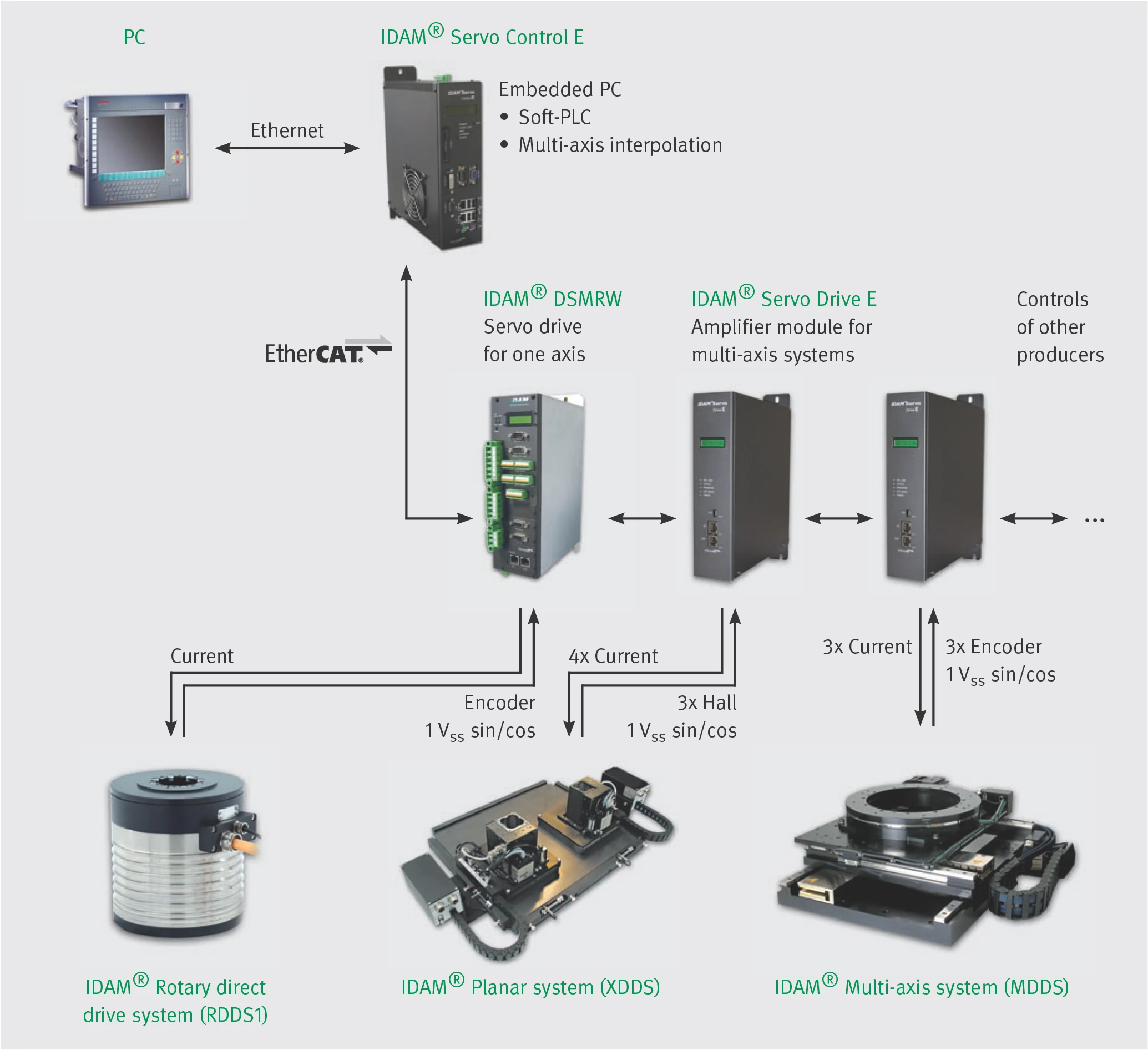
System configuration: RDDS1, IDAM DSMRW, Servo Control E, Servo Drive E and PC (Ethernet/EtherCAT) interconnection, supporting XDDS planar systems and MDDS multi-axis systems
The rotary direct drive system (RDDS1) can be operated with the following control architectures:
- IDAM® DSMRW: servo drive for one axis, or controls of other producers
- Current feedback
- Encoder 1 Vss sin/cos
- IDAM® Servo Control E + IDAM® Servo Drive E (amplifier module for multi-axis systems)
- Ethernet connection to PC (Embedded PC with Soft-PLC and multi-axis interpolation)
- Supports IDAM® RDDS1 (rotary), IDAM® XDDS (planar), IDAM® MDDS (multi-axis) systems
- Controls of other producers
Additional Loads
The following images show possible loading cases of the rotary system. External forces respectively additional masses cause certain loadings at the rotary system depending on point of application and position.
Axial Force and Axial Load
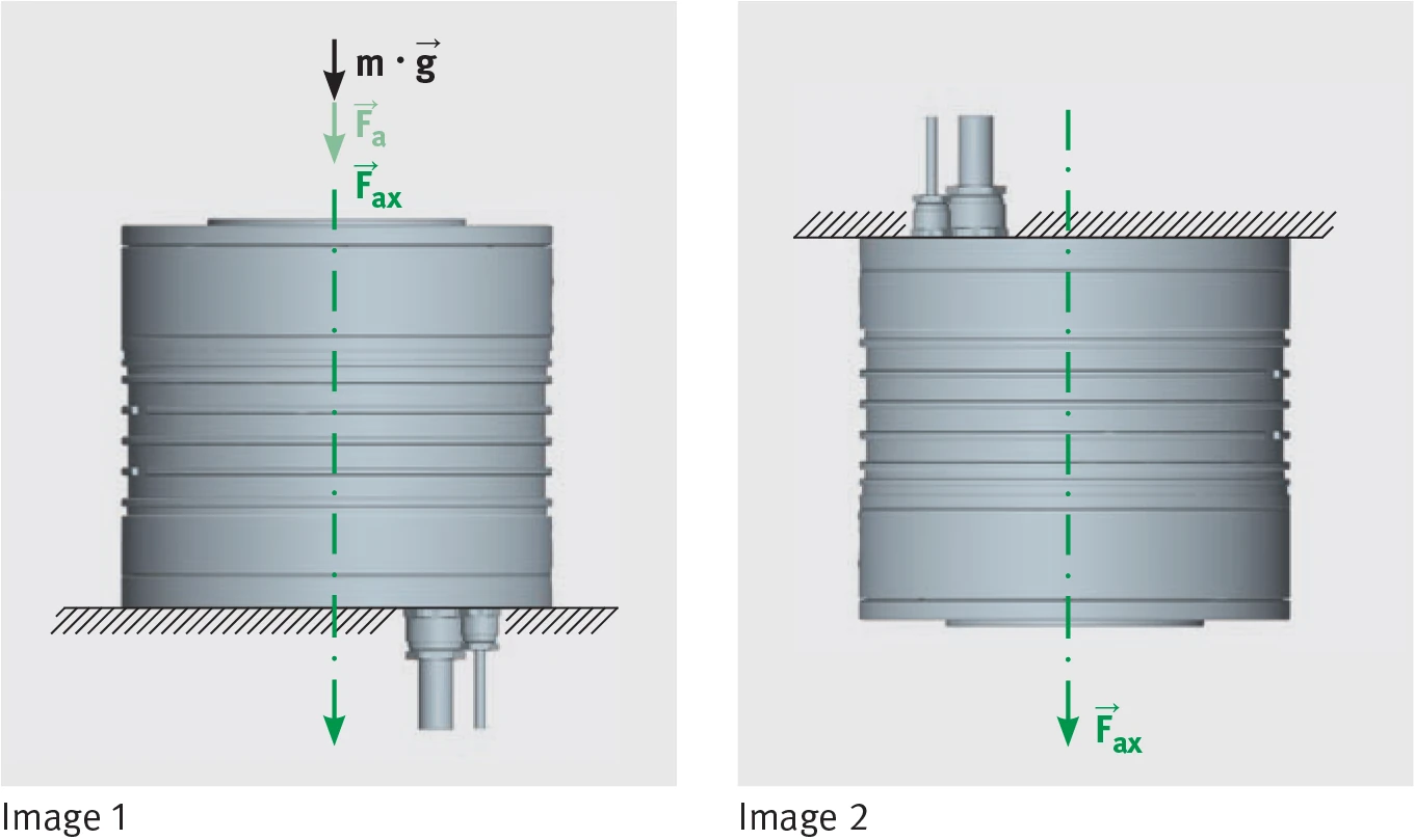
Image 1 and Image 2: resulting axial force Fax = Fa + m × g for centrical arrangement (two assembly orientations)
External forces affecting in the centre, whose line of action is identical with the rotary axis (Fa), as well as centrically arranged additional masses (m), lead to a resulting axial force (Fax) if the rotary systems are assembled like at image 1 and image 2:
Fax = Fa + m × g
Tilting Torque (Axial Eccentricity)
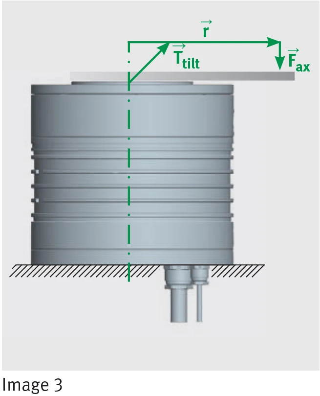
Image 3: eccentricity r generating tilting torque Ttilt (upright mounting)
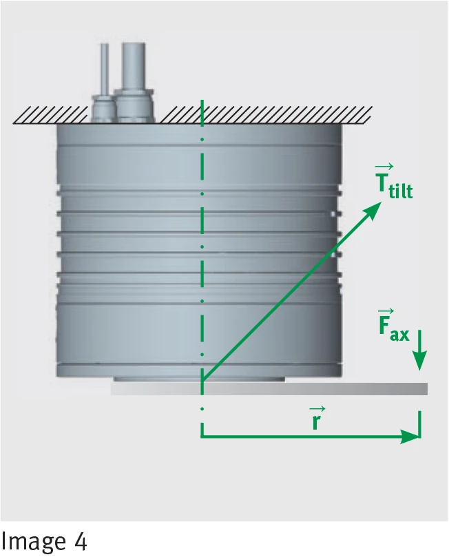
Image 4: eccentricity r generating tilting torque Ttilt (inverted mounting)
If the resulting axial force (Fax) is eccentric to the rotary axis with the distance (r) (images 3 and 4), the rotary system is strained by an additional tilting torque:
Ttilt = r × Fax
In case of lever arm and force being perpendicular to each other:
|Ttilt| = |r| × |Fax| × sin 90°
Ttilt = r × Fax
Radial Force and Tilting Torque
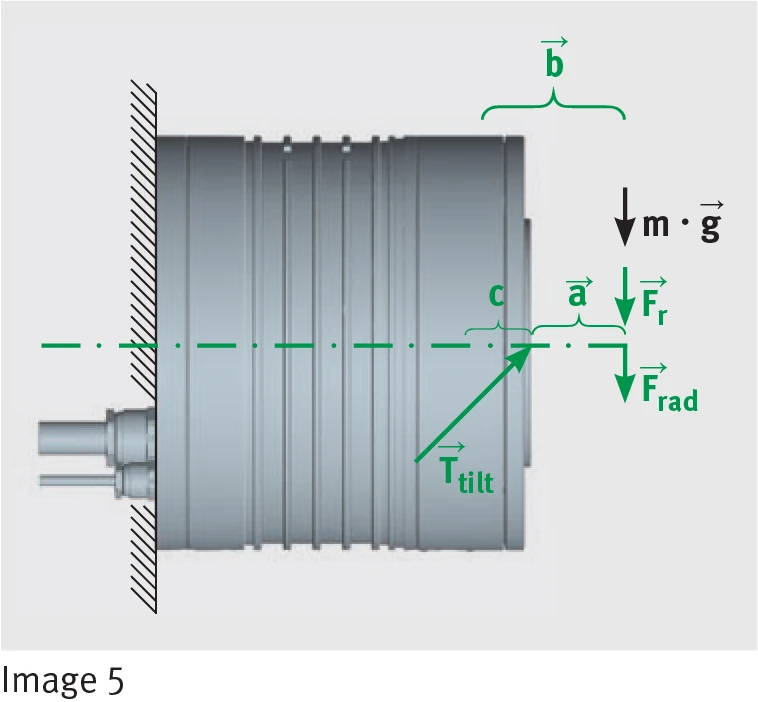
Image 5: radial force Fr, resulting radial force Frad, distances a, b, c and tilting torque Ttilt (horizontal mounting)
External forces (Fr), radially affecting the centre, whose line of action is perpendicular to the rotary axis, as well as centrically arranged additional masses (m), lead to a resulting radial strain (Frad) if the rotary systems are assembled like at image 5:
Frad = Fr + m × g
The point of application of the radial force (Frad) is generally at a distance (a) from the stage plate and the radial load leads additionally to a strain of tilting torque. The tilting torque is according to image 5:
Ttilt = b × Frad
If lever arm and force are perpendicular to each other, the tilting torque is analog to the above:
|Ttilt| = |b| × |Frad| × sin 90°
Ttilt = b × Frad
The distance b is according to image 5:
b = a + c
From this it follows the tilting torque:
Ttilt = (a + c) × Frad
c is a particular value for any diameter step:
| RDDS1 | c [m] |
|---|---|
| 130xH | 0.028 |
| 160xH | 0.032 |
| 180xH | 0.026 |
| 230xH | 0.029 |
Note: It is important that in no constellation one of the specified limiting values (Fax, Frad, Ttilt) are exceeded. Please contact us if you have higher demands regarding the loads.
Selection of Direct Drives for Rotary Applications
Cycled Applications
In cycled operation, sequential positioning movements are interspersed with pauses during which no motion takes place. A simple positioning sequence takes the form of a positively accelerated motion followed by a deceleration (negative acceleration of usually the same magnitude, in which case acceleration and deceleration time are equal). The maximum angular speed ωmax is reached at the end of an acceleration phase.
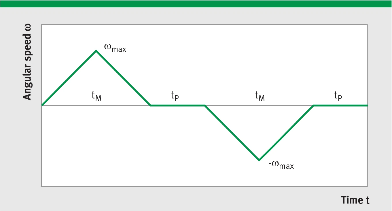
Angular speed ω vs. time t: showing ωmax, −ωmax, motion time tM and pause time tP for cycled forward-backward movement
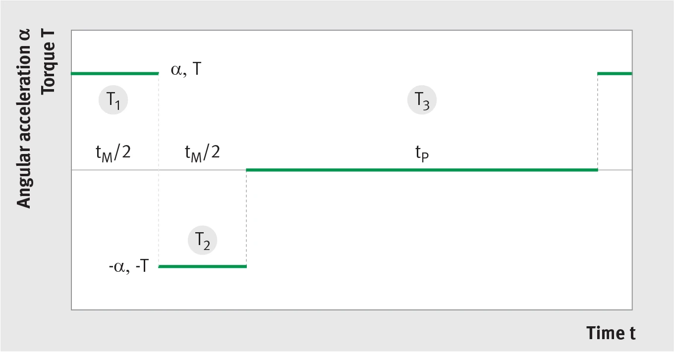
This gives the following α(t)-diagram (α: angular acceleration) as well as the flow of the torque required for the movement:
T = J × α
(T: torque [Nm], J: mass moment of inertia [kgm2], α: angular acceleration [rad/s2])
A cycle is described in the ω(t)-diagram (ω: angular speed, t: time). The diagram shows a forward-backward movement with pauses (tM: motion time, tP: pause time).
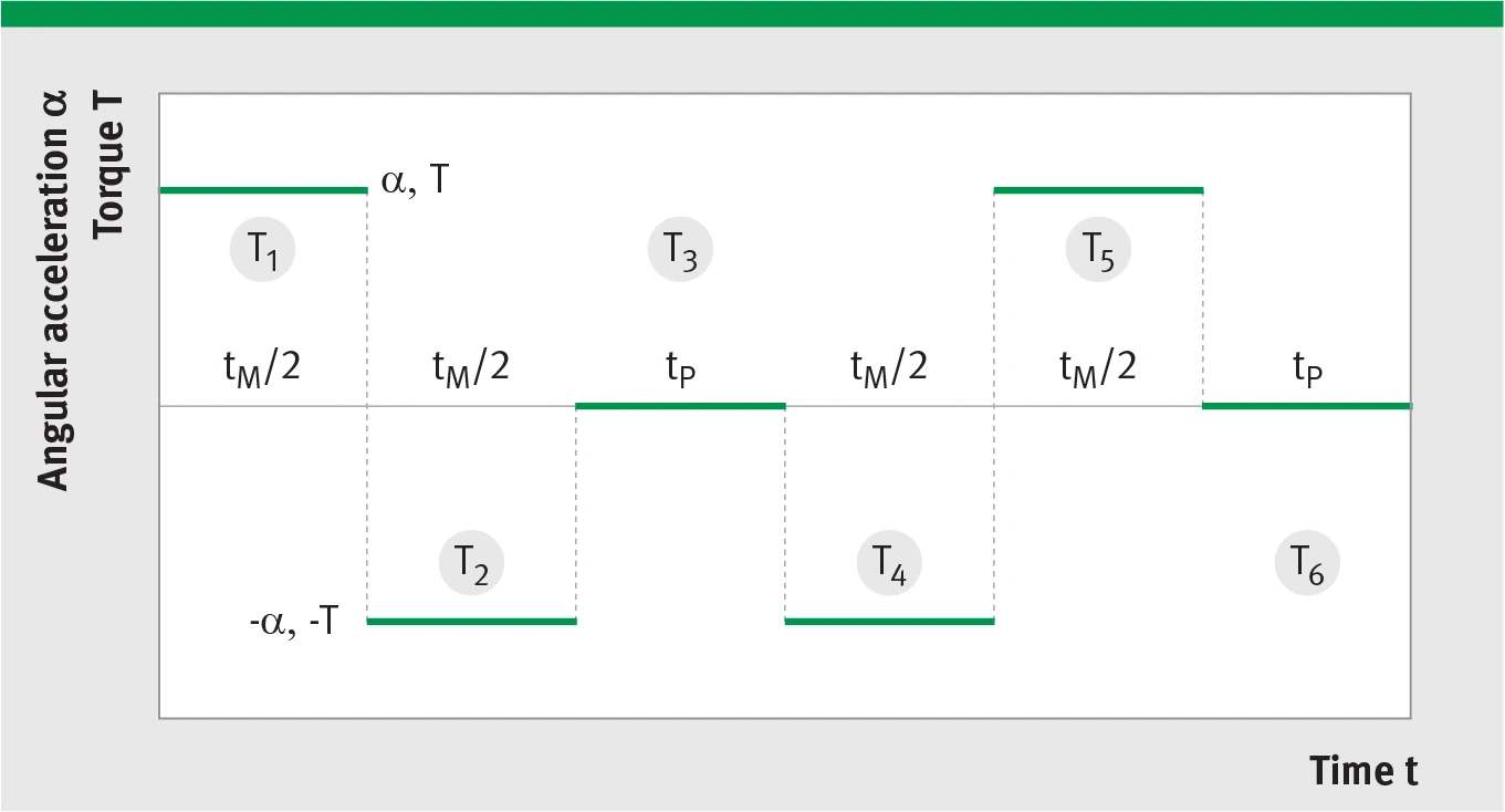
Angular acceleration α and torque T vs. time t: T1–T6 six torque cycles, showing tM/2 and tP time segments
According to the torque flow of the desired rhythm cycle, the motor is selected according to three criteria:
- Maximum torque in the cycle M: Tp (peak torque) according to data sheet
- Effective torque in the cycle M: Tc (motor uncooled) or Tcw (water cooling) according to data sheet
- Maximum rotary speed in the cycle M: nlp according to data sheet
The effective torque equals the root mean square of the torque curve (six torque cycles) in the rhythm cycle:
Trms = √T12·t1 + T22·t2 + … + T62·t6t1 + t2 + … + t6
The safety factor 1.4 in the sample calculation also takes into account the operation of the motor in the non-linear region of the torque-current characteristic, for which the formula for calculating Teff only applies approximately.
With the torques T1 = T; T2 = −T; T3 = 0; T4 = −T; T5 = T; T6 = 0 and the times t1 = tM/2; t2 = tM/2; t3 = tP; t4 = tM/2; t5 = tM/2; t6 = tP, the effective torque is calculated:
Trms = Tnom × √tMtM + tP
This equation is applied to the effective torque if torques of the same magnitude act in the rhythm cycle (mass moment of inertia and angular accelerations are constant). Below the root sign appears: "sum of the motion times divided by the total of the motion and pause times". The denominator is thus the cycle time.
Angular acceleration, maximum angular speed and maximum rotary speed of a positioning movement are calculated with:
α = 4 × φ / tM2
ωmax = α × tM / 2
nmax = 60 / (2 × π) × ωmax
| Symbol | Description | Unit |
|---|---|---|
| φ | Motion angle (positioning angle) | rad |
| tM | Motion time | s |
| α | Angular acceleration | rad/s2 |
| ωmax | Maximum angular speed | rad/s |
| nmax | Maximum rotary speed | rpm |
If a jerk limit is programmed in the servo-inverter, the positioning times extend accordingly. Constant positioning times require, in this case, greater accelerations.
Selection of Rotary Direct Drive Systems
Example: cycle applications, e.g. for test systems
| Preset values | Value | Description |
|---|---|---|
| Mass moment of inertia J [kgm2] | 0.018 | |
| Motion angle φ [°] | 22.5 | |
| Friction torque Tf [Nm] | 2 | |
| Installation space D (max. outer diameter) [mm] | 180 | |
| Motion time tM [ms] | 30 | |
| Safety factor | 1.4 | |
| Pause time tP [ms] | 60 |
Conversion of motion angle to radians:
φ = 180/π × 22.5° = 0.3927 rad
Calculation steps:
α = 4 × 0.3927 rad / (0.03 s)2 = 1745.33 rad/s2
ωmax = 1745.33 rad/s2 × 0.03 s / 2 = 26.18 rad/s
nmax = 60 / (2 × π) × 26.18 rad/s = 250 rpm
Together with the friction torque and the safety factor, this yields the maximum safety factor torque:
Tnom = [(0.018 kgm2 × 1745.33 rad/s2) + 2 Nm] × 1.4 = 46.78 Nm
In that case the torques for acceleration and braking are equal. The effective torque equals the root mean square of the torque curve (six torque cycles) in the rhythm cycle:
Trms = 46.78 Nm × √0.03 s0.03 s + 0.06 s = 27.01 Nm
(6 torque cycles equate 2 cycles)
System Selection Result
Both selected systems achieve the maximum rotary speed of 250 rpm.
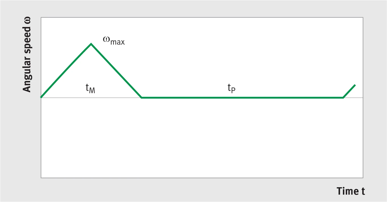
Selection example: angular speed ω vs. time t (ωmax, tM, tP)
Selection example: angular acceleration α and torque T vs. time t (T1–T3 simplified cycle)
Queries and Selection
For queries and selection of your application please do not hesitate to contact us.