Interactive Service Life L Calculator
Compute L (and optionally Lh) from your inputs
Dynamically Equivalent Load P Calculator
Feeds P into the L calculator above
Service Life Formulas
The formulas for calculating service life
For rollers and needles
For balls
a = Event probability factor
Ceff = Effective load carrying capacity per rolling element (N)
P = Dynamic, equivalent load (N)
L = Nominal service life (m)
Event probability factor a
Event probability factor a
The load carrying capacities for roller-contact bearings correspond to the DIN ISO standard. This represents a value from the service life calculation which is exceeded with a probability of 90 % during operational use of the guideway.
If the theoretical service life probability factor of 90 % mentioned above is not adequate, the service life value must be adjusted by a factor a.
| Event probability in % | 90 | 95 | 96 | 97 | 98 | 99 |
|---|---|---|---|---|---|---|
| Factor a | 1 | 0.62 | 0.53 | 0.44 | 0.33 | 0.21 |
Effective load carrying capacity Ceff
Effective load carrying capacity Ceff
External influences such as track hardness and temperature can reduce the loading capacity C, which means that Ceff needs to be calculated.
Ceff = Effective load carrying capacity per rolling element (N)
fH = Hardness factor
fT = Temperature factor
C = Max. permissible load carrying capacity per rolling element (N)
Hardness factor fH
Hardness factor fH
Materials in a frictionless guideway which deviate from the standard conditions (HRC 58–62) can be recorded with the factor fH:
| Track hardness in HRC | 20 | 30 | 40 | 50 | 55 | 56 | 57 | 58-62 |
|---|---|---|---|---|---|---|---|---|
| Hardness factor fH | 0.1 | 0.2 | 0.3 | 0.6 | 0.8 | 0.88 | 0.95 | 1 |
Temperature factor fT
Temperature factor fT
Increased temperatures influence the operating conditions (material properties) and must be taken into account using the factor fT.
| Temperature of the guideway in °C | 150 | 200 | 250 | 300 |
|---|---|---|---|---|
| Temperature factor fT | 1 | 0.9 | 0.75 | 0.6 |
Example calculation for Ceff
Example calculation for Ceff
Given:
- Guideway type R6
- Hardness 58–62 HRC ⇒ fH = 1
- Temperature 200°C ⇒ fT = 0.9
- Cage AA 6 ⇒ C = 530 N per roller
Dynamically equivalent load P
Dynamically equivalent load P
The loads (F) acting on a linear guideway system are subject to frequent fluctuations during operation. This set of circumstances should be taken into account when calculating service life. The varying load absorption of the guideway at varying operating conditions during the travel distance is described as the dynamic equivalent load P.
Stepped load
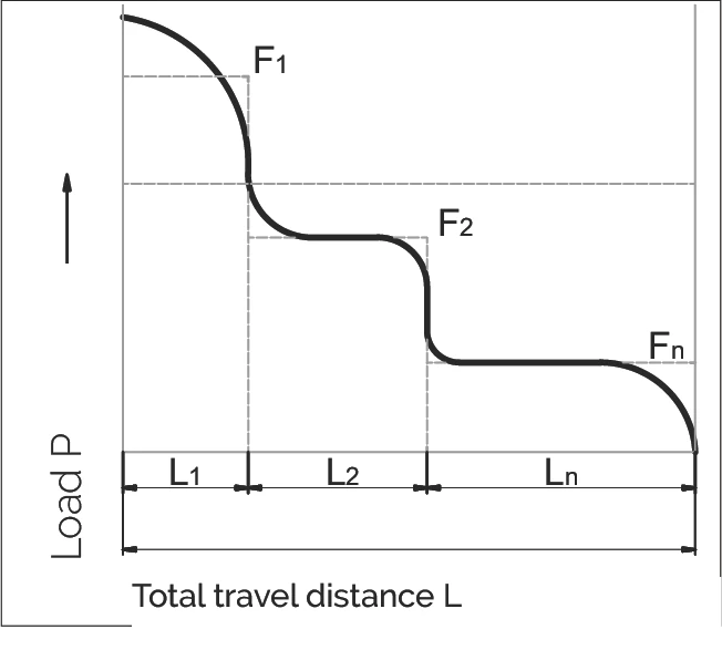
For rollers and needles:
For balls:
Sinusoidal load
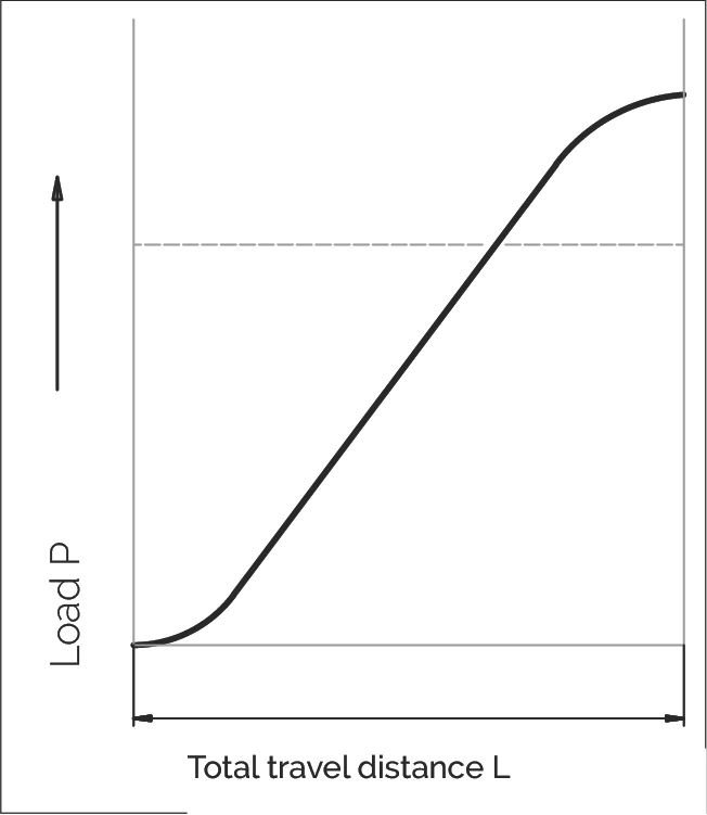
P = Equivalent load (N)
F₁...Fn = Individual load (N) during the partial travel distance L₁...Ln
Fmax = Max. load (N)
L = L₁ + ... + Ln = total travel during one load cycle (mm)
L₁...Ln = partial travel distance (mm) of an individual load during a load cycle
Service Life Calculation Example
Service Life Calculation Example
Example: Linear guideway RNG 6-300 with KBN 6 cage
Example calculation with a linear guideway of type RNG 6-300 with KBN 6 cage
1. Given Conditions
| Event probability | 97 % → factor a = 0.44 |
| Dynamic load capacity per roller | 1,800 N |
| Number of rollers | 16 |
| Total guideway load capacity | 16 × 1,800 N = 28,800 N |
| Applied load | P = 10,000 N |
2. Service Life Calculation (in meters)
Formula:
Substituting the values:
Result:
L = 1,495,412 m
Service life ≈ 1.5 million meters
3. Conversion to Operating Hours
To express service life in hours the following parameters must be known:
- H = stroke distance per cycle (m)
- t = time required to complete one stroke (s)
Formula for service life in hours:
Notes:
• The 3,600 in the denominator converts seconds to hours
• Lh is expressed in hours
• This formula assumes constant motion speed and load conditions
Correction factor Rtmin Helper
R_tmin Determination Helper
The correction factor Rtmin
The correction factor Rtmin
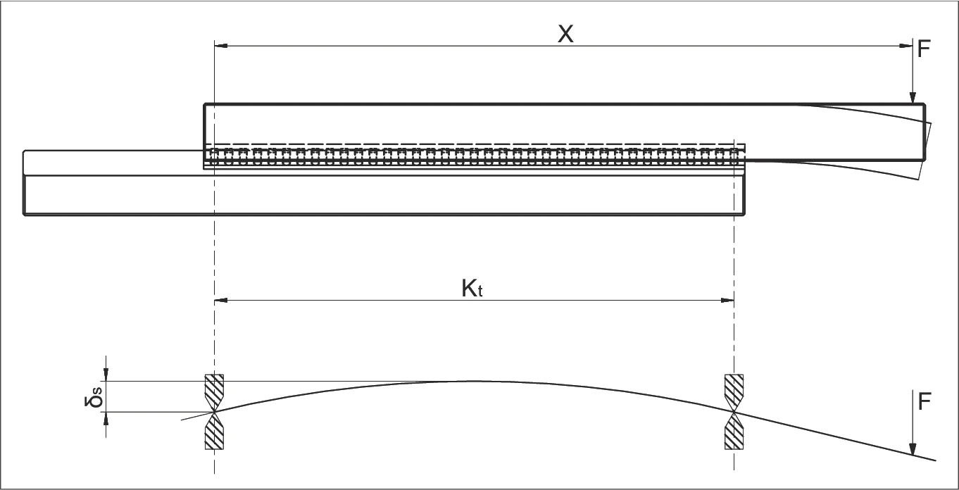
The previous sections explained how the service life is calculated from a given load carrying capacity and the actual load. In doing so, the number of load-bearing rolling elements per cage (Rt) must be taken into account.
Equally important is estimating the behavior of the surrounding structure when transmitting forces to the frictionless guideway. Elastic deformation or geometric errors in the machine tool cause only a portion of the installed rolling elements to effectively absorb load.
Reliable statements on this application-specific issue can usually only be made with a great deal of difficulty — for example by taking measurements on functional models or through calculations based on the finite element method. The result is that dimensioning is normally carried out using simplified measures, i.e. the external load is distributed onto fewer rolling elements using the correction factor Rtmin.
Determining Rtmin
Determining Rtmin
To determine Rtmin, the stiffness of the connecting structure must first be assessed based on historical experience:
A = Rigid structure
B = Normal structure
Parameter definitions
Parameter Definitions
| Symbol | Description | Unit |
|---|---|---|
| δS | Deformation of the connecting structure | µm |
| δA | Deformation of the rolling element including the guide rail (see chapter 12.5) | µm |
| F | Load | N |
| X | Lever arm distance on the x-axis | mm |
| Kt | Load-bearing cage length | mm |
| Rt | Number of load-bearing rollers | — |
| Rtmin | Correction factor | — |
Rtmin calculation chart
Chart for Calculating Rtmin
Chart notes:
- Curve A: Rigid structure
- Curve B: Normal structure
- Horizontal axis: X/Kt ratio
- Vertical axis: Rt values (Rt/2, Rt/4, etc.)
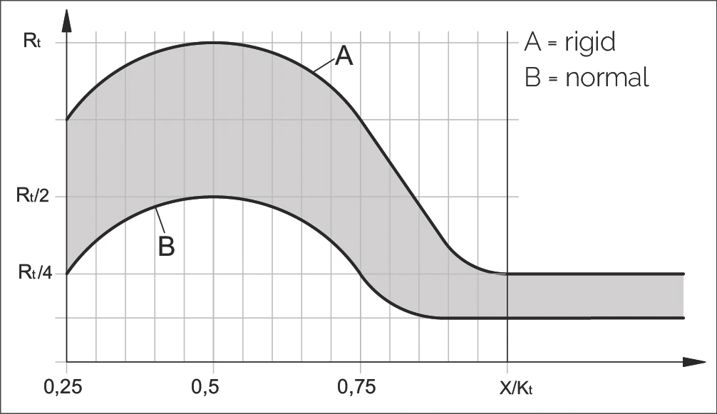
Calculating Rtmin from the diagram
To calculate Rtmin according to the diagram applies
| Structure | A (rigid) | B (normal) |
|---|---|---|
| X > Kt | Rtmin to Rt/4 | Rtmin |
| X < Kt | as per diagram | as per diagram |
Rtmin values for different rolling element types
Rtmin Values for Different Rolling Element Types
| Rtmin | Rolling element type | Cage types |
|---|---|---|
| 2 | Balls | AK |
| 1 | Rollers | AA, AC, EE, KBN and KBS |
| 5 | Needles | SHW and HW |
| 0.5 | Recirculating unit with rollers | SR and NRT |
| 1 | Recirculating unit with balls | SK, SKD and SKC |
Calculation examples
Calculation Examples
Example calculation no. 1: Linear guideway R6 with cage type AK 6/20
Example calculation no. 1: Linear guideway R6 with cage type AK 6/20
Given:
- X = 200 mm
- Kt = 171 mm
- Consequently the calculation method X > Kt applies
Analysis:
The linear guideway is horizontally arranged, therefore:
Calculation for a rigid structure
- According to the table, a ball count of Rtmin to Rt/4 applies
- Rtmin corresponds to 2 balls
- Rt/4 corresponds to 2.50 balls
Calculation for a normal structure
- According to the table, Rtmin applies
- Rtmin corresponds to 2 balls
Example calculation no. 2: Linear guideway R6 with cage type AK 6/11
Example calculation no. 2: Linear guideway R6 with cage type AK 6/11
Given:
- X = 75 mm
- Kt = 90 mm
- Consequently the calculation method X < Kt applies
Calculation for a rigid structure
According to the diagram, X = 0.83 of Kt (75 mm : 90 mm), consequently Rt/2
With 11 load-bearing balls this results in 5.5 balls (11 load-bearing balls : 2)
Calculation for a normal structure
According to the diagram Rt/8
With 11 load-bearing balls this results in 1.3 balls (11 : 8)