1.1 Legend of symbols used in formulas
Note
The table below lists all symbols, units and descriptions used in the formulas and diagrams of this chapter, 58 entries in total.
| Symbol | Unit | Description |
|---|---|---|
| I | A | Motor current |
| Ic eff | A | Effective continuous current, not cooled |
| Ic red | A | Reduced continuous current |
| Icw eff | A | Effective continuous current, cooled |
| Icw2 eff | A | Effective continuous current for higher speeds in continuous operation |
| Ip eff | A | Effective peak current |
| Ipl eff | A | Effective peak current, linear range |
| Iu eff | A | Effective ultimate current |
| J | kg·m² | Mass moment of inertia |
| km | Nm/√W | Motor constant for torque motors |
| kT | Nm/A | Torque constant |
| n | min⁻¹ | Speed |
| nlc | min⁻¹ | Limiting speed at Ic eff and UDCL |
| nlp | min⁻¹ | Limiting speed at Ip eff and UDCL |
| nlw | min⁻¹ | Knee speed |
| nlw2 | min⁻¹ | Operating speed FS at Icw2 eff and UDCL |
| nlw3 | min⁻¹ | Limiting speed at Icw2 eff and UDCL in continuous operation |
| nlwS1 | min⁻¹ | Rated speed S1, cooled |
| nmax | min⁻¹ | Max. speed |
| Pl | W | Power loss |
| Pmax S1 | N | Maximum rated power |
| R | Ω | Ohmic resistance |
| t | s | Time |
| T | Nm | Torque |
| tb | s | Pause time |
| Tc | Nm | Continuous torque, not cooled |
| Tcw | Nm | Continuous torque, cooled |
| Tcw2 | Nm | Torque at Icw2 eff and nlw2 |
| Tcw3 | Nm | Torque at Icw2 eff and nlw3 |
| Teff | Nm | Effective torque |
| TF | Nm | Bearing frictional torque |
| tm | s | Movement time |
| Tmax | Nm | Max. torque |
| Tp | Nm | Peak torque |
| Tpl | Nm | Peak torque, linear range |
| Tsafe eff | Nm | Effective torque, incl. safety factor |
| Tsafe max | Nm | Max. torque, incl. safety factor |
| Tsw | Nm | Stall torque, cooled |
| Tu | Nm | Ultimate torque |
| TW | Nm | Processing torque |
| TZ | Nm | Weight force (additional torque) |
| UDCL | V | DC link voltage |
| α | rad/s² | Angular acceleration |
| αmax | rad/s² | Max. angular acceleration |
| αS1 | rad/s² | Angular acceleration in S1 operation |
| ϑ | °C | Temperature |
| ϑf | °C | Current feed temperature |
| ϑmax | °C | Max. permissible winding temperature |
| ϑn | °C | Nominal response temperature |
| ϑnf | °C | Nominal feed temperature |
| φ | ° | Movement angle |
| ω | rad/s | Angular velocity |
| ωmax | rad/s | Max. angular velocity |
1.2 Advantages of torque motors
1.2.1 Performance capability
No conversion of the movement profile
There is no elasticity, play, friction or hysteresis in the drive chain resulting from transmission or coupling elements.
Multi-pole motor
Extremely high torques are produced as a result of the multi-pole design. The torques can be used from the speed > 0 up to the rated speed.
Thin, ring-shaped secondary part
The thin, ring-shaped design with a large, free inner diameter reduces motor inertia and yields a high acceleration rate.
Direct position measurement
High-precision, dynamic positioning operations are possible courtesy of the direct position measurement and rigid mechanical structure.
Controller compatibility
Torque motors from Schaeffler Industrial Drives can be operated with all common servo drives on the market.
1.2.2 Operating costs
No additional moving parts
The absence of additional moving parts makes assembly, adjustment and preventive maintenance of the drive unit easier.
Minimal wear in the drive chain
The drive chain is extremely durable even under very high alternating loads. The low amount of wear reduces machine downtimes.
High availability
In addition to the increased life and reduced wear, the robust design of the torque motors also increases the availability of the entire machine.
Energy efficiency
The heat is reduced to a minimum to save energy in the servo drive and cooler.
1.2.3 Design
Hollow shaft
The hollow shaft with large diameter makes the integration or passage of other assemblies possible, such as shafts, rotary distributors and media lines. Bearing level, force generation and effective working area can all be in close proximity to each other.
Installation of the primary part (stator)
The ring for the stator can be easily integrated into the machine construction due to the small space requirement.
Low section height
A highly compact and axially short construction with a high torque is made possible by the large, free inside diameter.
Few components
The highly engineered design makes it easier to incorporate the motor components into the machine assembly. The small number and robust design of the parts decreases the failure rate and increases the mean time between failures.
1.3 Characteristics of torque motors
A torque motor is made up of a primary part and a secondary part. The primary part contains an active coil system. The secondary part contains a permanent magnet system. In a concentric arrangement, the secondary part may either be the inner ring, in the case of an inner secondary part motor, or the outer ring, in the case of an outer secondary part motor. An energised primary part generates a force that acts on the secondary part as a result of the electromagnetic force.
A bearing maintains the air gap between the primary part and the secondary part. A measurement system for detecting the secondary part position is also required. Due to the wide range of application requirements, motor series have been developed with a wide variety of primary parts and secondary parts.
In terms of their structural design, torque motors can essentially be divided into motors with or without lamination stack or ironless motors. Further distinctions include the position and configuration of the secondary part as internal rotor or external rotor, or according to the magnet system. For example magnets can be glued on the surface of a steel ring, like they are in the RIB series. Or they can be integrated in a lamination stack – also referred to as buried magnets – in the RKIB series. The motors generate a consistently high torque over a wide speed range. The torque is determined by the active air gap area between the primary part and the secondary part as well as the structure. The designer must select the motor assemblies according to the power requirements. Conventional electric motors are classified according to power. Torque motors, by contrast, are classified according to the necessary torque.
Table 1: Characteristics of torque motors
| Motor series | Characteristics |
|---|---|
| RIB |
Internal running motor with high torque density
|
| RKI and RKIB |
Internal running motor with high power density
|
1.4 General motor characteristic values
1.4.1 Efficiency criteria
Power losses for torque motors are entered in the performance data according to winding and size. Although torque motors generate a high torque when stationary, they do not deliver any mechanical power. As a result, there is no reason to state the efficiency.
However, the motor constant km may be used for efficiency comparisons. The motor constant km defines the relationship between torque and copper loss generated at this torque. The power loss heats the motor. Furthermore, the motor constant km is accurate for the linear control range in a stationary state and at low speeds as well as at room temperature.
When the motor is subjected to a temperature increase, its efficiency decreases due to the increase in winding resistance. For speeds at a pole change frequency of 100 Hz or higher, the copper losses are joined by iron losses in the form of frequency dependent hysteresis losses and eddy current losses. Although the iron losses are not included in the motor constant km, they are relevant in the limiting speed range and should therefore be observed. The motor constant km only relates to the linear range of the torque–current characteristic curve.
Formula 1: Power loss
Pl = ( T / km )2
| Symbol | Unit | Description |
|---|---|---|
| Pl | W | Power loss |
| T | Nm | Torque |
| km | Nm/√W | Motor constant |
The motor constant km is dependent on the ohmic resistance and thus on the motor winding temperature. The motor constant km is stated in the performance data for +20 °C. The characteristic curve shows the motor constant as a function of the temperature.
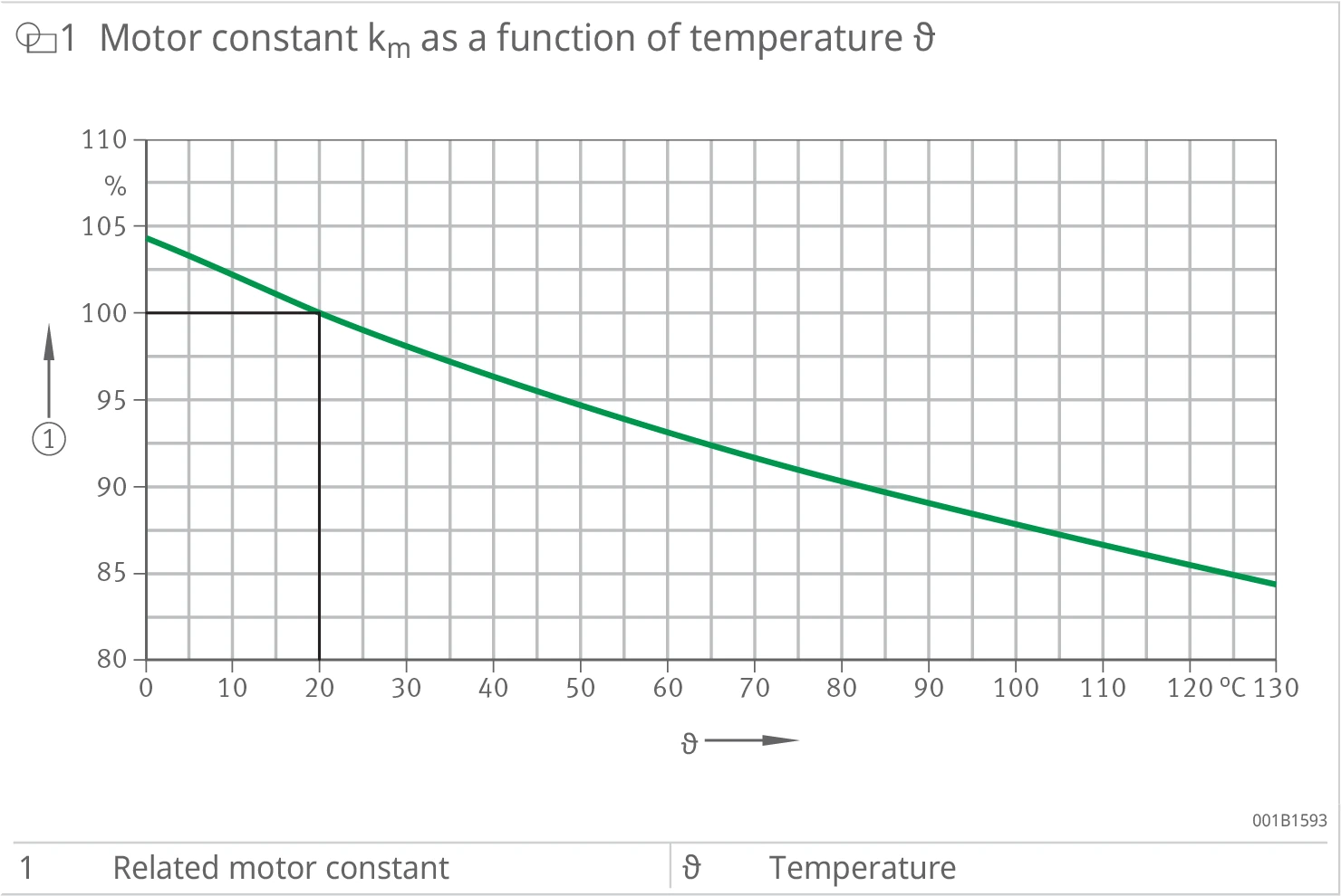
Figure 1: Motor constant km as a function of temperature ϑ. The vertical axis is the relative motor constant (%), the horizontal axis is temperature ϑ (°C). The curve is at 100% for +20 °C, decreasing as temperature rises, falling to about 84% at +130 °C. ①=related motor constant, ϑ=temperature.
Thermal behaviour
An increase in temperature brings about an increase in winding resistance, which has the effect of reducing the motor constant km. At +130 °C, the motor constant km falls to 0.84 times its normal value. At a constant current, which in turn generates the torque, a higher power loss occurs in the heated motor than in the cold motor. This power loss further increases the motor temperature.
1.4.2 Winding designs and dependencies
First and foremost, the series determines the limiting speeds of a torque motor. The following designs are possible:
- RIB torque motor: The primary part has a laminated iron core. For the secondary part, magnets are glued onto a steel ring.
- RKI torque motor and RKIB torque motor: The primary part has a laminated iron core. For the secondary part, magnets are integrated into the laminated core.
Within a series, the size, the DC link voltage and the winding design affect the limiting speeds.
Voltage drops within the motor increase the voltage requirement with increasing speed. At the knee speed specified in the performance data, the voltage requirement corresponds to the DC link voltage of the servo converter with field-oriented control, after which the speed falls off rapidly. The higher the DC link voltage and the smaller the voltage constants associated with the winding kû, the higher the achievable limiting speeds. As there is a correlation between voltage constant and torque constant, the power requirement of the motor increases with higher speed requirements at the same torque. One or more standard windings are predefined for different limiting speeds and dynamic requirements at a fixed DC link voltage UDCL.
1.4.2.1 Change in DC link voltage
The DC link voltage affects the winding-specific speed limits. If the DC link voltage changes by maximum ±10 %, a proportionality between the DC link voltage and the speed limits can be assumed for the pre-selection of the motor. Exact speed limits for customer-specific DC link voltages are available through the application engineers as well as through the sales department of Schaeffler Industrial Drives.
At lower DC link voltages, the limiting speed decreases. A torque–current characteristic curve shows the torque at different operating points. The torque–speed characteristic curves show the relationship between torque and speed at various operating points.
The torque–speed curves are available as a data sheet from the application engineers and the sales department of Schaeffler Industrial Drives. Contact: sales-sid@schaeffler.com
1.4.3 Torque/speed characteristic curve
RIB torque motor
The torque–speed characteristic curve for a RIB torque motor shows the winding-specific speed limits as a function of the torque at a constant DC link voltage without field weakening. The characteristic curve does not describe the duty cycle and the associated thermal behaviour of the motor. The characteristic curve only represents the range that the motor can approach at a winding temperature of +20 °C.
Operating points at torques in excess of Tcw are subject to time restrictions in order to protect the primary part from overheating. At Tu, an excessively high secondary part output temperature can lead to demagnetisation.
At n > nlwS1, the motor may only be operated for a specific amount of time due to additional frequency-dependent losses. Alternatively, the current can be reduced for continuous operation. The rated speed (S1), cooled, nlwS1, can also be equal to nlw depending on the motor size and winding design.
The limiting speed nlc at Ic eff and Tc is important for understanding the characteristic curve, but is not stated in the performance data due to its minor relevance.
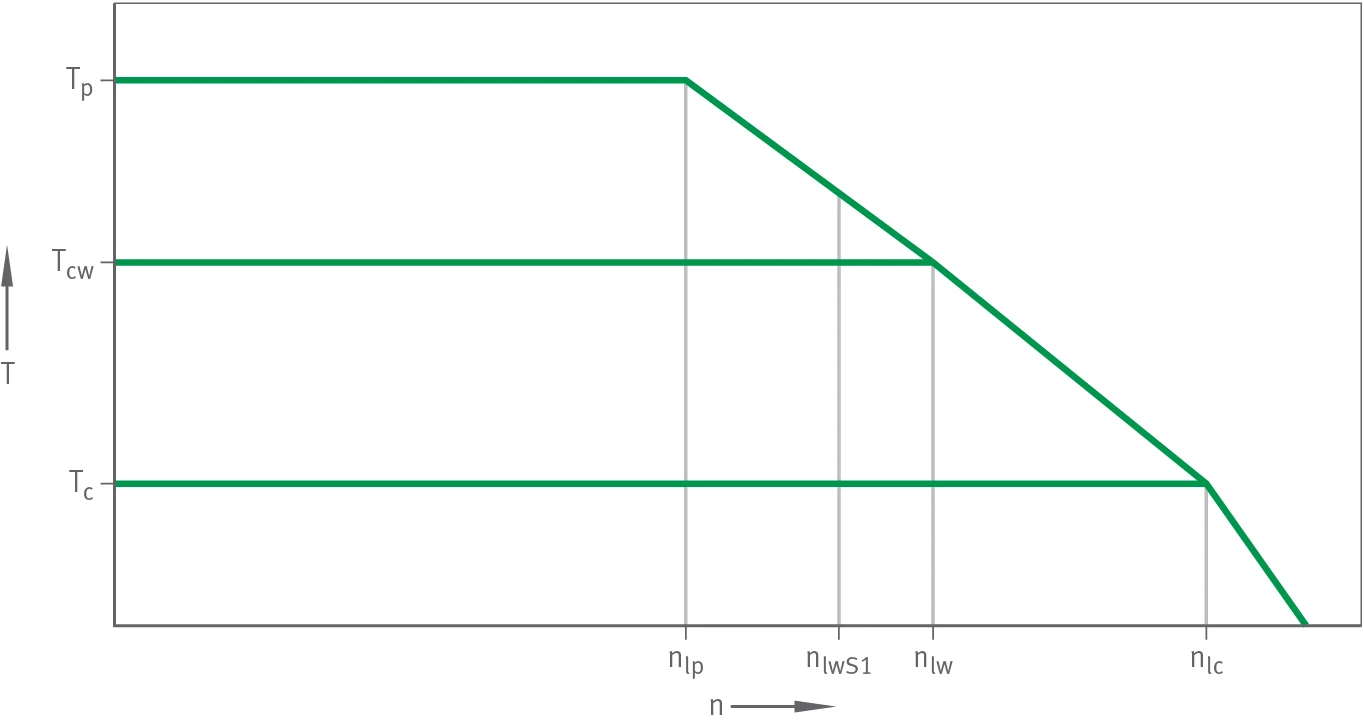
Figure 2: RIB torque motor: Torque–speed characteristic curve. The vertical axis is torque T, the horizontal axis is speed n. The curve shows three torque levels Tp, Tcw, Tc with the corresponding speed limits nlp, nlwS1, nlw, nlc. Symbol definitions: T=torque, n=speed, Tc=continuous torque, not cooled, Tcw=continuous torque, cooled, Tp=peak torque, nlc=limiting speed at Ic eff and UDCL, nlp=limiting speed at Ip eff and UDCL, nlw=knee speed, nlwS1=rated speed S1, cooled.
RKI torque motor and RKIB torque motor
The torque–speed characteristic curve for continuous speeds shows the winding-specific speed limits as a function of the torque at high speeds and constant DC link voltage with field weakening. RKI torque motors and RKIB torque motors can operate continuously at the operating points shown in the characteristic curve.
Operation at the continuous torque Tcw is possible up to the speed nlwS1. At higher speeds up to the speed nlw2, continuous operation requires a reduction in current from Icw eff to Icw2 eff. The associated torque is Tcw2.
Between nlw2 and nlw3, the maximum permissible continuous current is also Icw2 eff. The associated torque progression depends on the winding and the secondary part configuration. At nlw3 and Icw2 eff, the associated torque is Tcw3. The mechanical power at this operating point is Pmax S1. The precise progression between nlw2 and nlw3 can only be seen in the product-specific data sheet, which must be requested from Schaeffler Industrial Drives.
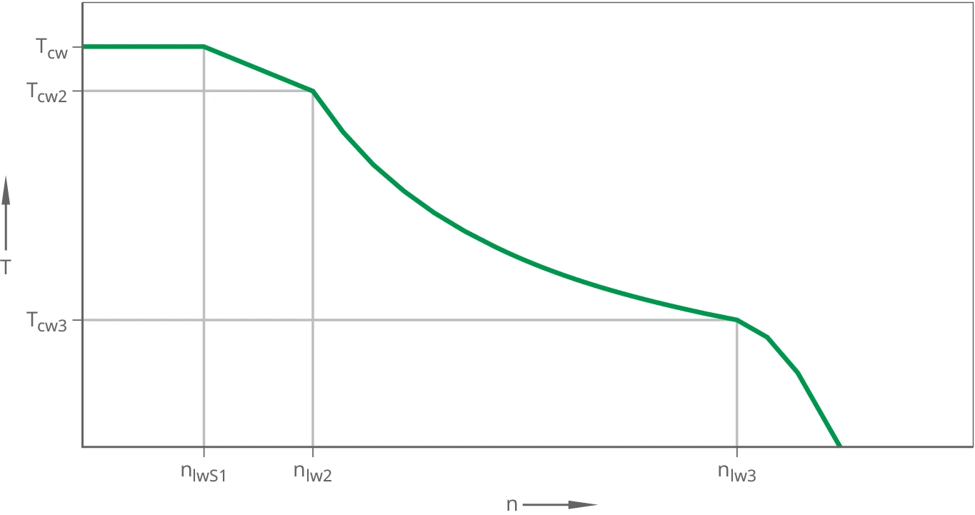
Figure 3: RKIB torque motor: Torque–speed characteristic curve for continuous speeds. The vertical axis is torque T, the horizontal axis is speed n. The curve shows Tcw, Tcw2, Tcw3 with the corresponding speed limits nlwS1, nlw2, nlw3. Symbol definitions: n=speed, T=torque, Tcw=continuous torque, cooled, Tcw2=torque at Icw2 eff and nlw2, Tcw3=torque at Icw2 eff and nlw3, nlwS1=rated speed S1, cooled, nlw2=operating speed FS at Icw2 eff and UDCL, nlw3=limiting speed at Icw2 eff and UDCL in continuous operation.
Control reserve: All specified speeds relate to a constant DC link voltage UDCL. With frequency inverters without a stabilised DC link, UDCL is not constant. The operating point must therefore be provided with a control reserve as a function of the DC link voltage fluctuation. Typically, with frequency inverters without a stabilised DC link, the speed at the operating point should not exceed approx. 80 % of the motor's possible speed at this operating point.
1.4.4 Torque/current characteristic curve
A motor current in the range between 0 A and the linear peak current Ipl eff generates a linearly dependent torque. The peak current Ipl eff generates the linear peak torque Tpl. The motor constant km is suitable for calculating the power loss in the range between 0 A and Ipl eff. The torque constant kT is used in this range to calculate the torque on the basis of the current, or vice versa.
The value of the linear peak current Ipl eff is independent of temperature. The value depends on the series and the winding design. It can be lower or higher than the value of the cooled continuous current Icw eff. The linear peak current Ipl eff and the associated linear peak torque Tpl are important for understanding the characteristic curve. However, as these values have very little practical relevance, they are not listed in the performance data.
The torque–current characteristic curve is no longer linear at I > Ip eff. The saturation of a motor's magnetic circuits causes this non-linearity. Between the torque–current points Tp at Ip eff and Tu at Iu eff, the characteristic curve becomes non-linear. In this range, the gradient of the curve is variable and significantly lower than the value of the torque constant kT.
The motor can be operated for a few seconds up to the operating point Tp, Ip eff. This is the maximum operating point for acceleration processes. Due to the risk of demagnetisation of the permanent magnets, the motor must not be operated beyond the limiting point Tu, Iu eff.
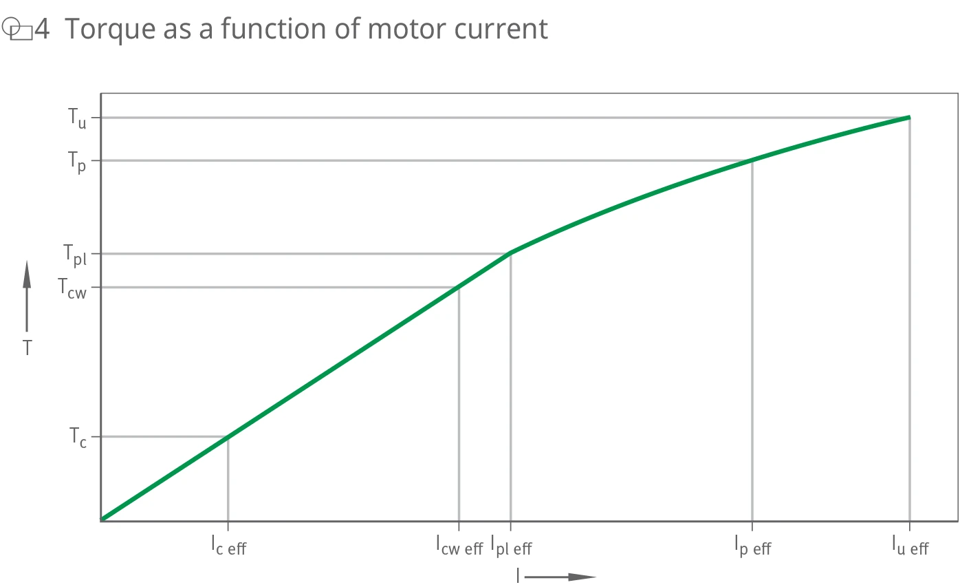
Figure 4: Torque as a function of motor current. The vertical axis is torque T, the horizontal axis is motor current I. The curve is linear between 0 and Ip eff, and becomes non-linear beyond it due to magnetic saturation, up to Tu, Iu eff. The torque levels Tc, Tcw, Tpl, Tp, Tu and current points Ic eff, Icw eff, Ipl eff, Ip eff, Iu eff are marked.
1.5 Thermal motor protection
1.5.1 Monitoring circuits I and II
Users often operate direct drives at their thermal performance limit. In addition, an unpredictable overload can occur during operation. The overload results in a current load that is higher than the permissible continuous current. In the event of overload, the effective motor current, the square mean value I²t, must not exceed the permissible continuous motor current. For short-term overcurrent, the power electronics must have an I²t motor protection model to control the motor current. This indirect temperature monitoring is very fast and reliable. During motor commissioning, the user must ensure that the I²t monitoring is switched on.
Motors from Schaeffler Industrial Drives must be protected by means of motor temperature monitoring. Monitoring circuit I of the standard version contains 3 PTC sensors, connected in series, on the 3 phase windings. Monitoring circuit II also includes a Pt1000 sensor on one phase in the motor. This sensor enables pre-warning thresholds.
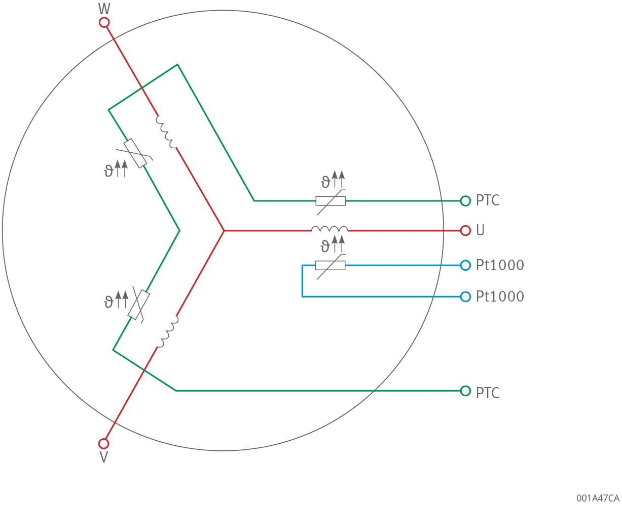
Figure 5: Standard connection of triplet PTC and Pt1000. Shows the connection terminal arrangement of 3 PTC sensors connected in series on the motor's three-phase U, V, W windings, and a Pt1000 sensor on one phase.
The PTC and Pt1000 sensors have basic isolation from the motor. The sensors are not suitable for direct connection to PELV circuits or SELV circuits in accordance with DIN EN 61800-5-1.
1.5.2 Monitoring circuit I
A PTC is a thermistor. A PTC has a thermal time constant of a few seconds. In contrast to that of the Pt1000, the resistance of the PTC rises very sharply when the nominal response temperature ϑn is exceeded. The resistance increases to a multiple of the cold value when the nominal response temperature is exceeded.
When using a triple PTC, i.e. three PTC sensors connected in series, the total resistance changes significantly. This considerable change also occurs if only one sensor exceeds the response temperature ϑn. The use of three PTC sensors ensures that the motor can still be shut down safely by a thermistor motor protection relay under asymmetrical phase load, e.g. at standstill. The thermistor motor protection relay typically trips between 1.5 kΩ and 3.5 kΩ, thus triggering a controller stop.
The PTC sensors detect the overtemperature of each winding with a deviation of only a few degrees.
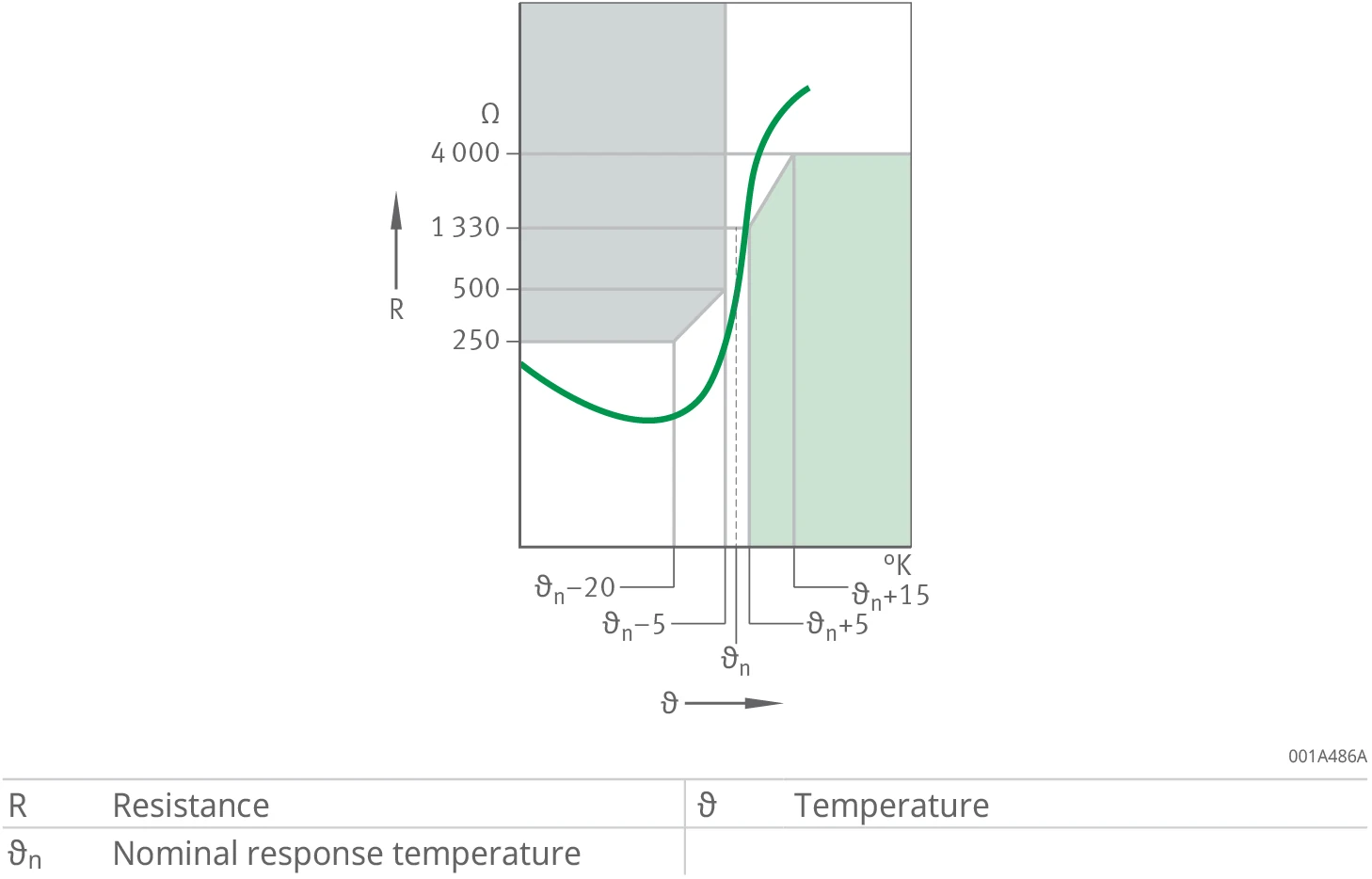
Figure 6: PTC temperature characteristics. The vertical axis is resistance R (Ω), the horizontal axis is temperature ϑ. The resistance is low below the nominal response temperature ϑn and rises sharply beyond it. The resistance levels 250, 500, 1330, 4000 Ω and temperature ranges ϑn−20, ϑn−5, ϑn, ϑn+5, ϑn+15 are marked. Symbol definitions: R=resistance, ϑ=temperature, ϑn=nominal response temperature.
The thermistor motor protection relay also responds if the resistance in the PTC circuit is too low. The excessively low resistance may indicate a defect in the monitoring circuit. The thermistor motor protection relay ensures safe galvanic isolation of the controller from the PTC sensors in the motor. The thermistor motor protection relay is not included in the scope of delivery of the motor. PTC sensors of temperature monitoring circuit I are not suitable for temperature measurements. Monitoring circuit II is suitable for temperature measurements.
In principle, a thermistor motor protection relay connected to the servo converter must evaluate the PTC sensors for temperature protection of the motor.
1.5.3 Monitoring circuit II
The Pt1000 is a platinum measuring resistor temperature sensor. This sensor makes use of the temperature dependence of the electrical resistance of platinum. EN 60751 describes the sensor characteristic.
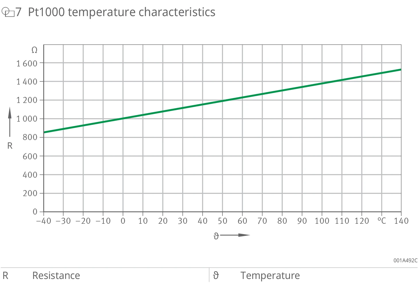
Figure 7: Pt1000 temperature characteristics. The vertical axis is resistance R (Ω), the horizontal axis is temperature ϑ (−40 to +140 °C). The curve rises linearly, from about 800 Ω (−40 °C) to about 1540 Ω (+140 °C). Symbol definitions: R=resistance, ϑ=temperature.
The thermal time constant is a few seconds in the installed state. Pre-warning threshold and a shutdown limit are entered in the controller and protect the motor from overtemperature. The pre-warning threshold prevents immediate shutdown by the thermistor motor protection relay.
At standstill, depending on the application, constant currents can flow through the windings of the motor. The pole position determines the magnitude of the constant currents. The motor is not heated homogeneously through this dependency. Unmonitored windings may overheat. A Pt1000 sensor can only monitor one phase. The use and evaluation of three Pt1000 sensors ensure the monitoring of all phases. For applications that regularly reach the loading limit at standstill, Schaeffler Industrial Drives recommends the use and evaluation of three Pt1000 sensors.
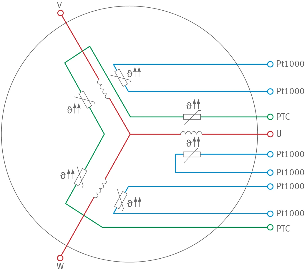
Figure 8: Connection of triplet PTC and 3 Pt1000. Shows the connection terminal arrangement of 3 PTC (in series) and 3 Pt1000 sensors on the motor's three-phase V, U, W windings.
1.6 Electrical connection technology
1.6.1 Standard cable connections
The standard cable connections of motors from Schaeffler Industrial Drives are equipped with an axial screw connection. For RIB torque motors, their relative position to the cooling connections is in the middle of the cable outlet. For RKI torque motors and RKIB torque motors with multiple cable outlets, the relative position cannot be universally defined. The quotation and delivery drawing and the 3D model take precedence and provide a binding position.
RIB torque motors are supplied with a 2 m cable. The cable length is measured from the motor outlet. RKI torque motors and RKIB torque motors are supplied with either a 2 m or a 5 m cable. Customised cable lengths are available.
The cross section of the power connection cable depends on the continuous current of the motor. As standard, dimensioning is based on the continuous current Icw eff at Plw (cooled). Axial, radial and tangential cable outlets can be used. The desired cable outlet is defined with the order. For motor currents over 70 A, the cable outlets are matched to the specific application.
The cables have the following characteristics:
- shielded
- resistant to oil and coolant courtesy of polyurethane outside surface
- flame resistant
- suitable for drag chain use
The cable ends are open with ferrules in the standard version. Application-specific cable outlets are possible.
Table 2: Motor cable connections, standard
| Cross-section | Continuous current | Diameter | min. bending radius, fixed | min. bending radius, flexible | Mass |
|---|---|---|---|---|---|
| – | A | mm | mm | mm | g/m |
| 4G0,75 | 10,4 | 8 | 40 | 80 | 95 |
| 4G1,5 | 16,1 | 9 | 45 | 90 | 140 |
| 4G2,5 | 22 | 10,5 | 52,5 | 105 | 210 |
| 4G4 | 30 | 12,5 | 62,5 | 125 | 296 |
| 4G6 | 37 | 14,5 | 72,5 | 145 | 416 |
| 4G10 | 52 | 17 | 85 | 170 | 644 |
| 4G16 | 70 | 20,5 | 102,5 | 205 | 997 |
Table 3: Motor connection assignments
| Designation | Assignment |
|---|---|
| 1/U | Phase U |
| 2/V | Phase V |
| 3/W | Phase W |
| GNYE | PE |
The sensor cable enables temperature monitoring with the PTC and Pt1000 sensors. The cable ends are open with ferrules in the standard version. Application-specific cable outlets are possible.
Table 4: Sensor cable connections, standard
| Cross-section | Temperature monitoring | Diameter | min. bending radius, fixed | min. bending radius, flexible | Mass |
|---|---|---|---|---|---|
| – | – | mm | mm | mm | g/m |
| Sensor 4×0,14 | P 1) | 4,8 | 24 | 36 | 40 |
| Sensor 7×0,14 | – | 5,7 | 29 | 43 | 67 |
| Sensor 10×0,14 | T 2) | 6,7 | 34 | 50 | 87 |
1) P = 1 Pt1000 + 3 PTC 2) T = 3 Pt1000 + 3 PTC
Table 5: Connection assignments, sensor variant P
| Designation | Assignment |
|---|---|
| WH | PTC |
| BN | PTC |
| GN | Pt1000 |
| YE | Pt1000 |
Table 6: Connection assignments, sensor variant T
| Designation | Assignment |
|---|---|
| WH | PTC |
| BN | PTC |
| GN | Pt1000-1 |
| YE | Pt1000-1 |
| GY | Pt1000-2 |
| PK | Pt1000-2 |
| BU | Pt1000-3 |
| RD | Pt1000-3 |
1.6.2 Special cable connections
For RKI torque motors and RKIB torque motors, the use of shielded single wires may make sense in certain cases. The selected wires and their positions can be found in the quotation and delivery drawings as well as the quotation circuit diagram. General characteristic values of the single wires can be found in the table.
Table 7: Motor cable connections, special designs
| Cross-section | Continuous current | Diameter | min. bending radius, fixed | min. bending radius, flexible | Mass |
|---|---|---|---|---|---|
| – | A | mm | mm | mm | g/m |
| 4×(1×2,5) | 22 | 4×6 | 24 | 45 | 4×58 |
| 4×(1×4) | 30 | 4×6,5 | 26 | 49 | 4×77 |
| 4×(1×6) | 37 | 4×7 | 28 | 53 | 4×101 |
| 4×(1×10) | 52 | 4×8,5 | 34 | 64 | 4×146 |
| 4×(1×16) | 70 | 4×10 | 40 | 75 | 4×223 |
| 4×(1×25) | 88 | 4×12 | 48 | 90 | 4×329 |
| 4×(1×35) | 110 | 4×13 | 52 | 98 | 4×444 |
1.6.3 Positive direction of rotation of the motor
The electrically positive direction of rotation corresponds to a clockwise rotating field in all three-phase motors, i.e. the phase voltages are induced in a U, V, W sequence. Motors from Schaeffler Industrial Drives have the following positive direction of rotation with secondary part movement:
- anticlockwise when viewing the side of the cable outlet from above
- clockwise when viewing the side facing away from the cable outlet at the bottom
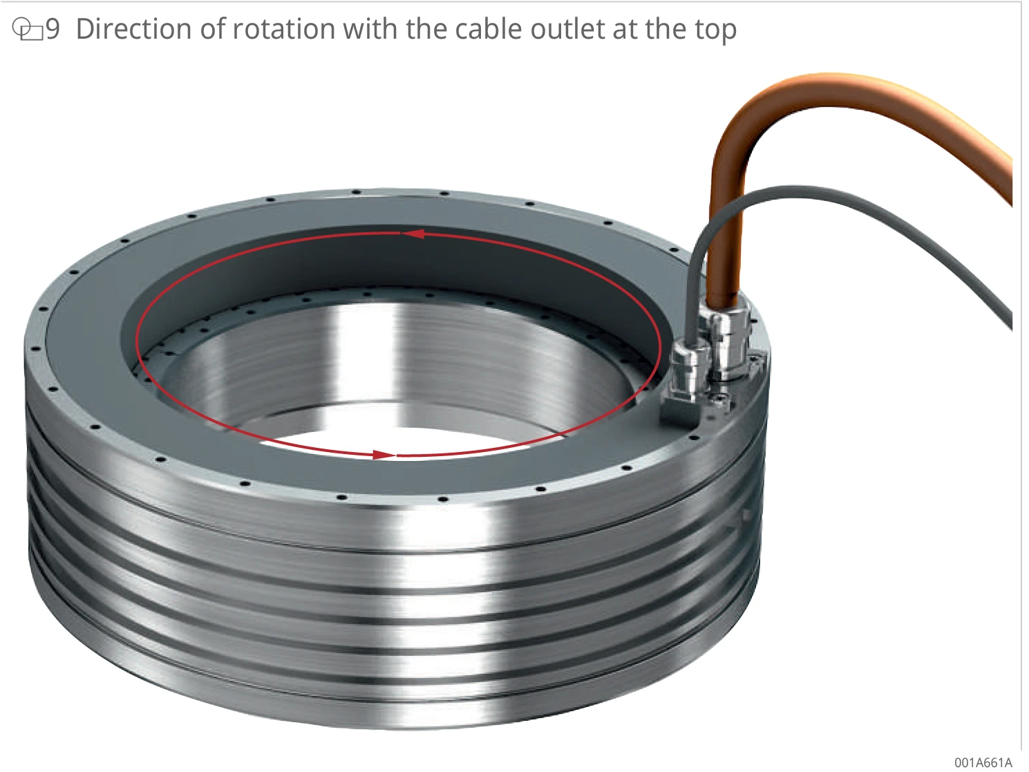
Figure 9: Direction of rotation with the cable outlet at the top. The motor photo marks the direction of rotation with secondary part movement (red arrow, anticlockwise).
1.6.4 Commutation
Synchronous motors should be operated with commutation where possible. Schaeffler recommends commutation that is based on the measuring system, since this is supported by modern servo drives and controllers.
1.6.5 Isolation strength and overvoltage phenomena
Schaeffler Industrial Drives develops, designs and manufactures motors according to the following directive: 2014/35/EU, Electrical equipment for use within certain voltage limits. The motors meet the requirements of the following directive: 2014/30/EU, Electromagnetic compatibility. The motors are intended to be used for the intended operation in a PDS (power drive system) in accordance with DIN EN 61800-5-1.
The insulation systems of the motors are designed to overvoltage category III and optimised for maximum life. The dielectric strength of the insulation systems is checked before delivery. Modern test methods, such as measuring the partial discharge inception voltage, ensure the life and performance of the motors over a long time period.
When installed, the motor is part of the PDS, which consists of the motor, motor cable and converter components such as the supply module, regenerative modules, drive controller and filter. Unwanted and unpredictable effects can occur within the PDS. Controller manufacturers often provide recommendations and project planning information that the user should observe and adhere to. Failure to do so may result in premature failure of the motor or converter insulation systems.
The following measures ensure safer operation, regardless of the converter:
- Short cables and large-area cable shielding support: Short cables and large-area support/contact of the cable screen help avoid overvoltages caused by high frequency reflection on the motor cable. Motor cables with lengths of 10 m or higher between the motor and the converter increase the probability of overvoltages. Schaeffler Industrial Drives recommends measuring the voltage on the motor connection terminals using a suitable high-voltage technology when the machine is put into operation.
- Selecting the right motor: The motors must be selected according to the DC link voltage of the converter. In most cases, the DC link voltage is 600 V. A lower DC link voltage reduces the dynamic response and maximum speed. A reinforced insulation system is required if the DC link voltage is 720 V or higher or the installation height is greater than 2000 m. In such cases, contact Schaeffler Industrial Drives. Motors with inductances well over 50 mH, measured from phase to phase, may only be used following individual checks by the manufacturer of the converter and Schaeffler Industrial Drives, as otherwise voltage spikes may cause resonances in the PDS (power drive system) and damage to the insulation system.
Instructions from the converter manufacturer must be observed. If any of the following applies, this must be specified in the request. Alternatively, measurement of the transient overshoot can be carried out during commissioning on site.
- PDS with multi-axis converter modules or regulated supplies: here, electrical oscillations relative to earth potential and the resulting voltage load can damage the motor's insulation system.
- Applications in which more pronounced insulation damage has occurred in the past
- Applications in which countermeasures already exist
For a DC link voltage of 600 V to 720 V, the overshoot between the motor phases must not exceed 1370 V. The peak-to-peak band between the motor phases must not exceed 2800 V.
Line reflections and electrical oscillations due to regulated supplies are superimposed in the measurement between motor phase and earth potential. Only the peak-to-peak band should be considered during the evaluation. The peak-to-peak band must not exceed 2350 V.
1.6.6 Short-circuit behaviour in permanent magnet synchronous motors
In an emergency, a short circuit of phases U, V and W can decelerate an axis driven by a torque motor. This emergency braking generates a short-circuit current. The magnitude and duration of the current load must be taken into account in the sizing of the PDS (power drive system). If the short-circuit current is higher than the cooled continuous current Icw, Schaeffler Industrial Drives must be consulted. The braking behaviour of the motor is calculated based on speed and moment of inertia.
1.7 Cooling and cooling circuit
1.7.1 Heat distribution
The motor assembly transmits the power loss that occurs during motor operation to the machine. The design measures implemented for cooling, convection, conduction and radiation can be used to influence and control the heat distribution of the overall system. Knowledge of the heat sources in a motor is decisive for the structural design.
At low speeds, and therefore pole change frequencies < 100 Hz, heat is generated solely by copper loss in the motor windings. At higher speeds, and thus pole change frequencies > 100 Hz, iron losses in the secondary part and primary part as well as magnet losses in the secondary part also occur. The iron losses do not increase linearly with the pole change frequency and depend on the field weakening angle and current density.
Most of the heat generated in operation at pole change frequencies < 100 Hz can be dissipated through a liquid cooling system on the outer surface of the primary part. The so-called jacket cooling system is connected to the cooling circuit of a recooler. The cooling jacket is usually a structural component of the customer-specific machine design, but can also be provided separately by Schaeffler Industrial Drives. The cooling medium travels through openings in the cooling ribs – the so-called cooling meander – across different levels from inlet to outlet. The inlet and outlet can be assigned to the two connections as desired. The flow area is sealed to the outside with O-rings.
For machines with high power density, high speeds, and therefore pole change frequencies > 100 Hz, excellent dynamic response or high accuracy, Schaeffler Industrial Drives additionally recommends the use of a temperature control system (heating or cooling) for the surrounding structure or the secondary part. A rotary manifold is typically used to cool the bearing and secondary part. Temperature control of the surrounding structure helps to minimise thermal distortion of the machine structure and the effect on the bearing preload, thereby increasing accuracy.
Continuous torques of torque motors with liquid cooling on the primary part are up to 300 % higher than in uncooled operation. To achieve high continuous torques, torque motors are operated with liquid cooling in most applications.
The design of motor cooling is influenced by the following factors:
- installation space
- accuracy requirements
- thermal sensitivity of the surrounding structure
- required speeds
1.7.2 Cooling media and their effect on cooling
The information in the performance data is based on water as the cooling medium. However, water requires additives that prevent corrosion and biological deposits in the cooling circuit. Use of a cooling medium that differs greatly from water has the effect of reducing the amount of heat that can be dissipated and thus also of changing the continuous torque, cooled Tcw, that is available in continuous operation. Upon request, Schaeffler Industrial Drives can provide help with sizing the application and determining the achievable motor data.
For sizing with a customer-specific cooling medium, the following information is required:
- type and density
- specific heat capacity
- kinematic viscosity
- technical data sheet with constituent substances
If cooling media with a significantly higher viscosity than that of water are used, the effect on the cooling must be checked before use. Motor parameters such as Icw eff or Tcw may need to be adjusted. Data for the medium used must be used and expected temperatures must be taken into account.
Water
Water is the most commonly used cooling medium. Water has a high specific heat capacity and is inexpensive. Water with additives that prevent corrosion and biological deposits is preferable to all other cooling media. Additives such as COOL CONCENTRATE or COOL X hardly affect properties such as density and viscosity. Water with one of these additives is a very efficient cooling medium with a specific heat capacity of 4.1 kJ/kg·K. This value approximately corresponds to the value for water.
Table 8: Material properties of water
| Temperature | Density 1) | Specific heat capacity | Dynamic viscosity | Kinematic viscosity |
|---|---|---|---|---|
| °C | kg/m³ | kJ/kg·K | Pa·s | mm²/s |
| +20 2) | 998,21 | 4,1840 | 0,0010014 | 1,00319572 |
| +25 | 997,05 | 4,1813 | 0,00088982 | 0,892452736 |
| +30 | 995,65 | 4,1798 | 0,00079705 | 0,800532316 |
1) According to DIN 1306, secondary conditions such as air pressure and gravitational acceleration apply 1 g, pressure pn = 1.01325 bar.
2) Reference temperature.
Water–glycol mixture
A mixture of water and glycol has a lower freezing point than that of water and prevents corrosion. This mixture is often used for cold environments or applications in which frost protection is required. Due to the higher viscosity of the water–glycol mixture compared with that of pure water, there is a higher pressure loss in the pipe system. The circulating pump must deliver a correspondingly higher pressure.
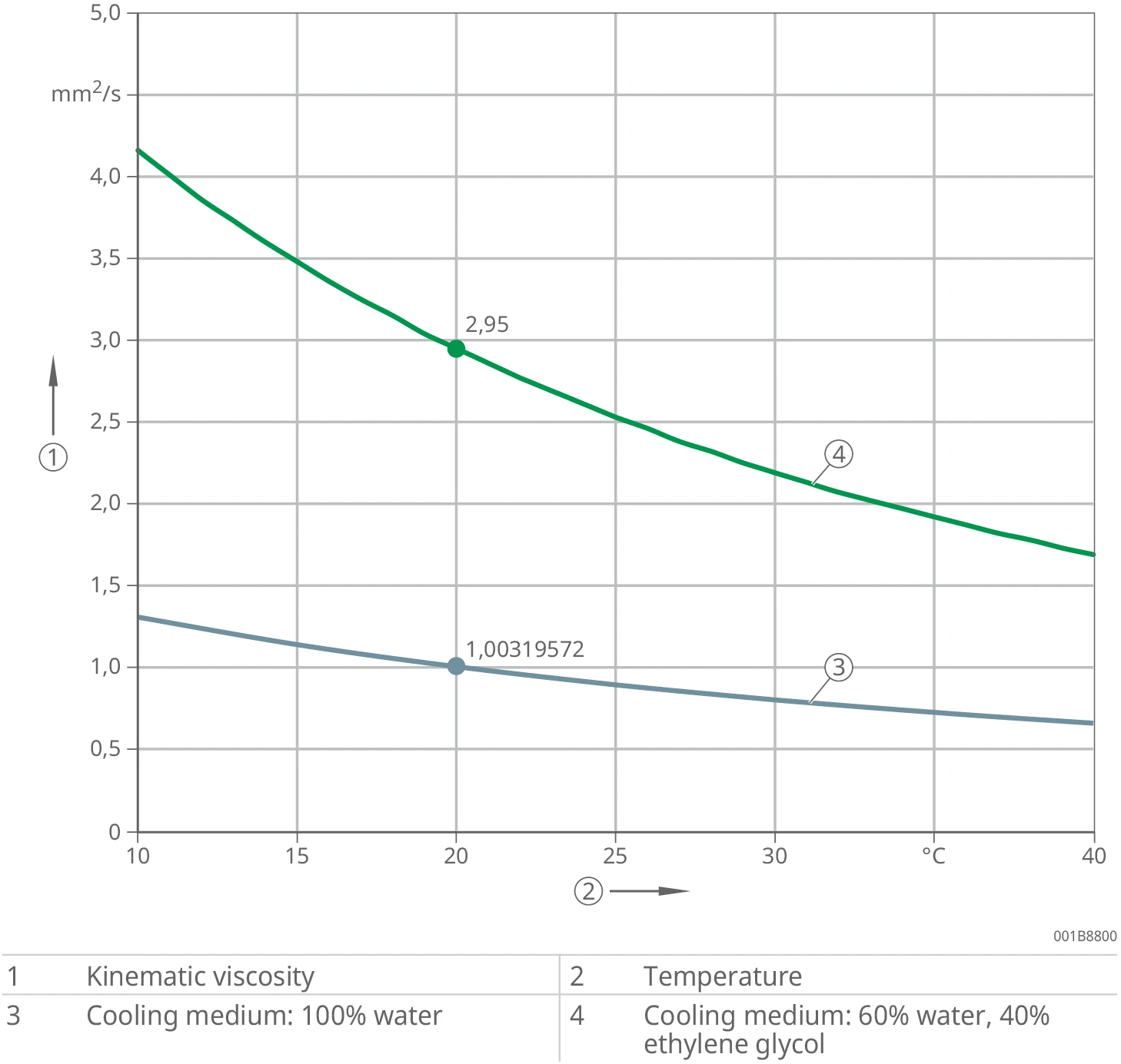
Figure 10: Dependence of kinematic viscosity on temperature. The vertical axis is kinematic viscosity (mm²/s), the horizontal axis is temperature (°C). Two curves: ③=cooling medium 100% water (1.00319572 at 20 °C), ④=cooling medium 60% water + 40% ethylene glycol (2.95 at 20 °C). Symbol definitions: ①=kinematic viscosity, ②=temperature.
Example
A mixture of 40 % ethylene glycol, e.g. Antifrogen N, and 60 % water has a freezing point of −25 °C and a kinematic viscosity that is 2.95 times higher than that of water. The recommended flow rate can only be achieved with a significantly higher pressure. Correction factors can be used for a rough estimate.
Table 9: Correction factors for ethylene glycol
| Concentration | Freezing point | Correction factor for pressure difference |
|---|---|---|
| % | °C | – |
| 20 | −9 | 1,14 |
| 30 | −16 | 1,23 |
| 40 | −25 | 1,33 |
| 44 | −30 | 1,38 |
The exact values for the cooling medium used must always be observed.
Oils
Oils are used as cooling media in some industrial applications. The application determines which oil is the right one. If oil is used, the volume flow necessary for cooling must always be achieved. Upon request, Schaeffler Industrial Drives can provide help with sizing. The chemical compatibility of all components must be checked by the customer.
1.7.3 Influence of nominal data on the supply temperature and cooling medium
The specified continuous current for cooled operation Icw eff refers to the nominal cooling water feed temperature ϑnf. The continuous current Icw eff is specified in the performance data.
Higher supply temperatures ϑf reduce the cooling capacity and, thus, also the continuous current. The reduced continuous current Ic red is calculated from the following quadratic relationship:
Formula 2: Reduced continuous current
Ic red / Icw eff = √(ϑmax − ϑf) / (ϑmax − ϑnf)
| Symbol | Unit | Description |
|---|---|---|
| Ic red | A | Reduced continuous current |
| Icw eff | A | Effective continuous current, cooled |
| ϑmax | °C | Max. permissible winding temperature |
| ϑnf | °C | Nominal feed temperature |
| ϑf | °C | Current feed temperature |
If customer-specific cooling media are used, the amount of waste heat that can be dissipated and, thus, also the cooled continuous torque that is available during continuous operation are changed. Upon request and with specification of the substance properties, engineers from Schaeffler Industrial Drives can determine the effect of the cooling medium used.
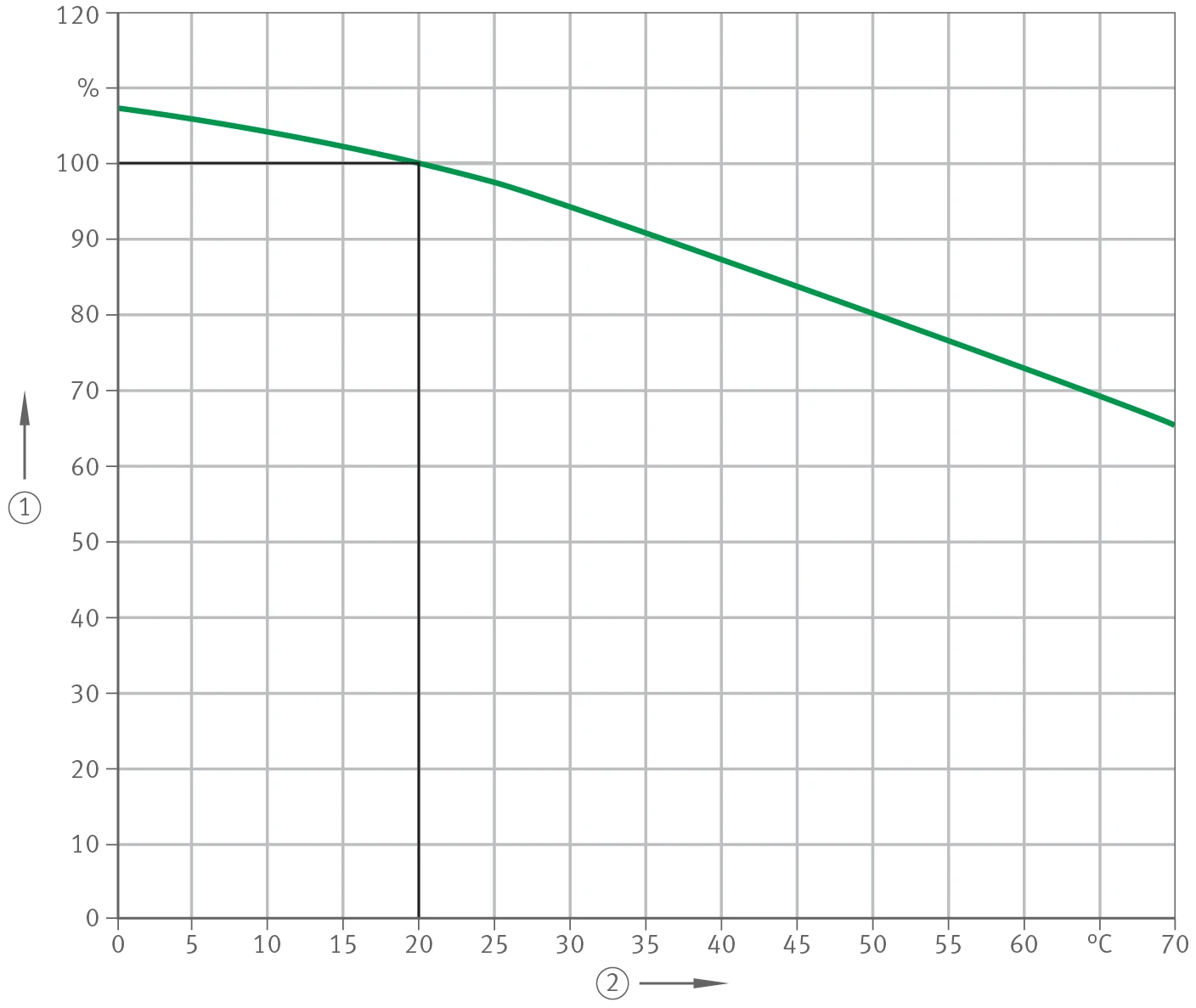
Figure 11: Relative continuous current Ic red / Icw eff as a function of supply temperature ϑf (ϑnf = +20 °C). The vertical axis is relative continuous current (%), the horizontal axis is actual supply temperature ϑf (°C). The curve is at 100% for +20 °C and decreases as the temperature rises. Symbol definitions: ①=relative continuous current Ic red / Icw eff in %, ②=actual supply temperature ϑf, Ic red=reduced continuous current, Icw eff=continuous current, cooled, ϑnf=nominal feed temperature.
1.8 Arrangement of motors
1.8.1 Operating several motors in parallel on one axis
Driving an axis simultaneously with 2 or more synchronous motors makes sense in some applications. Such applications include pivot systems in five-axis machining centres, fork-type milling heads or machine spindles for hobbing machines. Identically built synchronous motors connected in parallel can be operated together on a converter. Only low speeds allow for satisfactory synchronisation quality if two torque motors are operated in parallel on one axis. Therefore, in practice, only torque motors in the RIB series are used for parallel operation. RIB series torque motors are slower than RKIB series torque motors.
1.8.2 Arrangement of motors
A distinction is made between the parallel tandem arrangement and the anti-parallel, i.e. mirrored, Janus arrangement of the primary parts.
Secondary part alignment
In parallel operation, secondary parts must be aligned in the same angular position, regardless of the arrangement. The respective secondary part markings can be used for alignment.
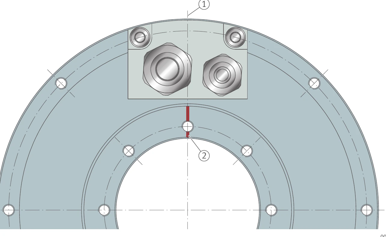
Figure 12: Zero axis and rotary markings in alignment. ①=zero axis, ②=secondary part (rotor) marking.
Primary part alignment
The aim is to align the coils of each phase in the same angular position. The primary part can be aligned using the zero axis. In a standard RIB motor with a single cable outlet, the zero axis is located between the holes on the cable clamp. In the case of customer-specific or multiple cable outlets, Schaeffler Industrial Drives must be consulted to determine the zero axis.
Before parallel operation can be planned, Schaeffler Industrial Drives must be contacted.
Tandem arrangement
The cable outlets point in the same longitudinal direction.
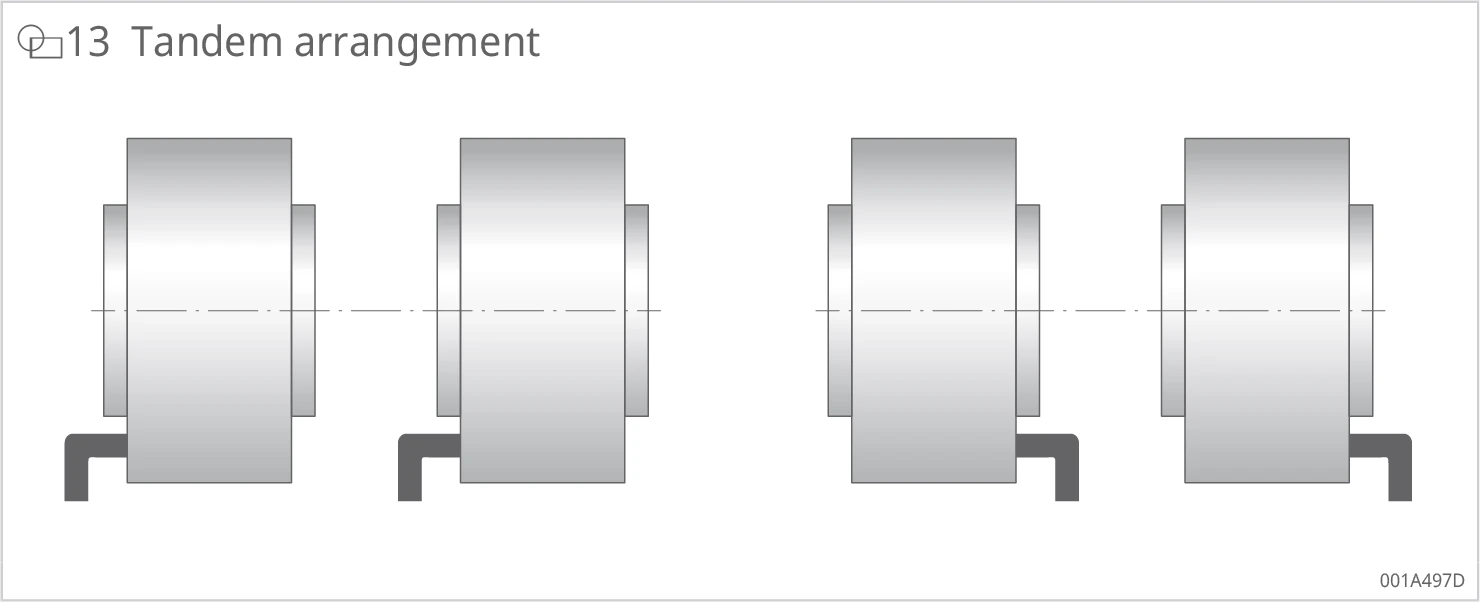
Figure 13: Tandem arrangement. Schematic of two pairs of motors with cable outlets pointing in the same longitudinal direction.
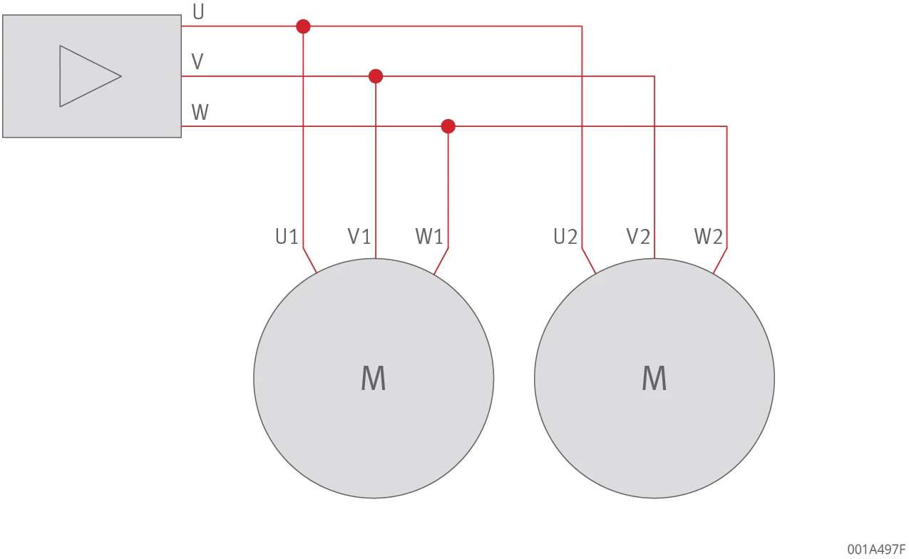
Figure 14: Tandem arrangement wiring diagram. The converter phases U, V, W are connected respectively to the U1/V1/W1 and U2/V2/W2 terminals of the two motors M (phases of the same name connected together).
The zero axes of the primary parts are also aligned with the cable outlets. In the case of flush coaxial cable outlets, the bolt circles must be concentrically arranged and the phase connections of the same names must be lined up.
Janus arrangement
The cable outlets point in opposite longitudinal directions.
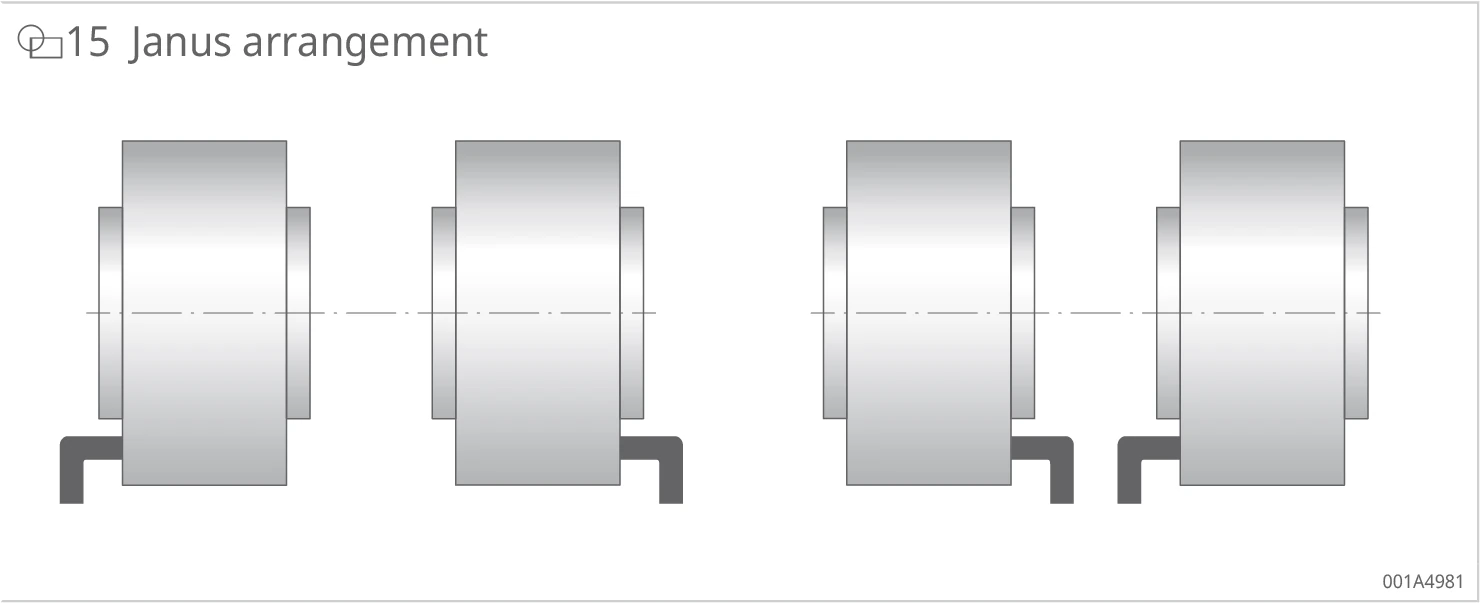
Figure 15: Janus arrangement. Schematic of two pairs of motors with cable outlets pointing in opposite longitudinal directions.
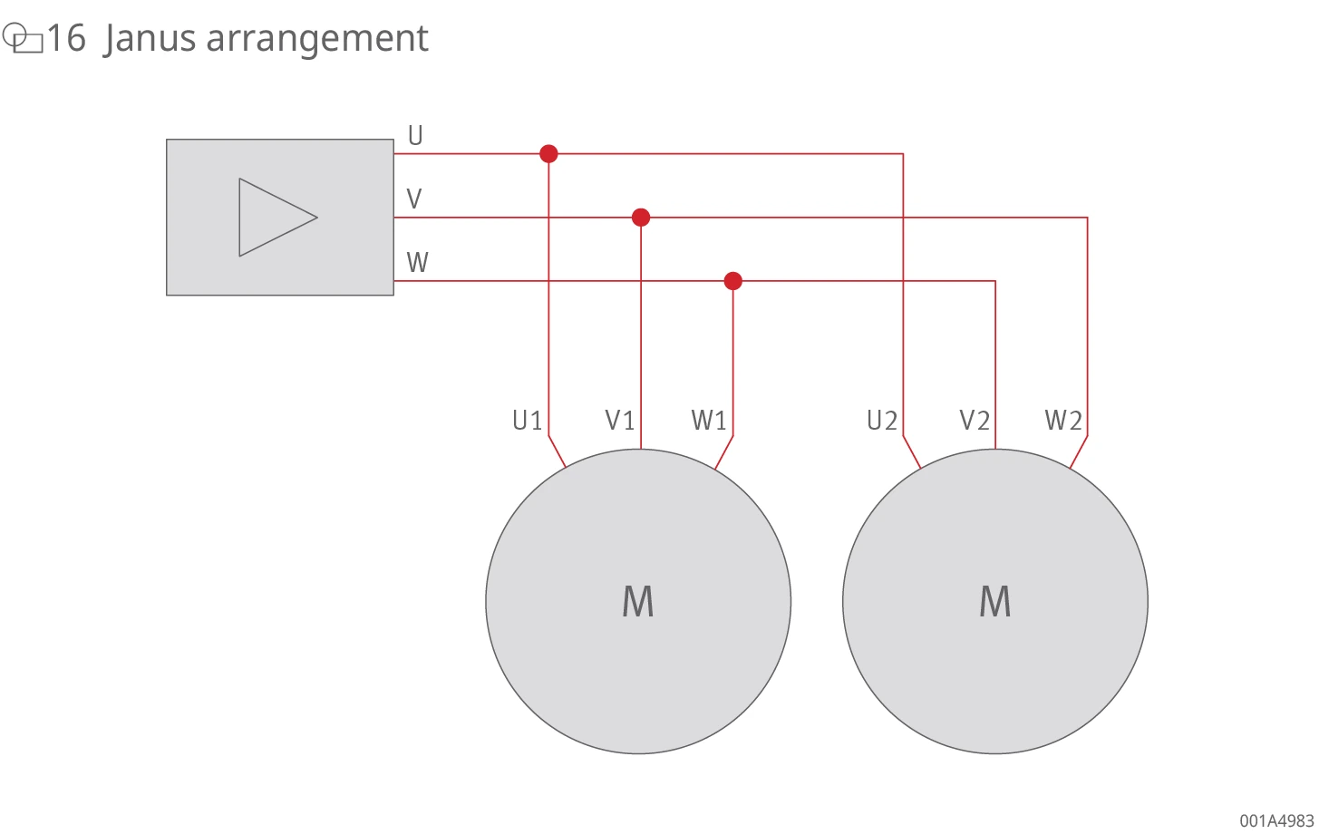
Figure 16: Janus arrangement wiring diagram. The converter phases U, V, W are connected to the two motors M, with the V and W phases of one motor interchanged to achieve mirrored operation.
The zero axes must also match in the mirrored Janus arrangement. Depending on the position of the zero axis, it may be necessary to offset the bolt circles. Motors in a mirrored arrangement must work in the opposite direction of rotation. For this purpose, the phases V and W are interchanged on one of the two motors. As a result, the phases U1 and U2, V1 and W2 and W1 and V2 are connected together to the converter.
1.9 Operating several motors in parallel on one axis
1.9.1 Displacement of the cable outlet
In all arrangements, the primary parts and thus the cable outlets can be twisted relative to each other in steps of a certain size. Particularly in the Janus arrangement with internal cable outlets, it is possible to design a shorter overall axis by twisting the primary parts. The step size corresponds to a pair of poles and must be multiplied by an integer factor.
The twist angle is calculated as follows:
Formula 3: Torsion angle
Torsion angle = ( 360° / Number of pole pairs ) · x
| Symbol | Unit | Description |
|---|---|---|
| x | – | any integer factor |
In some series, a favourable twist angle is also achievable in the bolt circle, e.g. RIB11-3P-230xH:
Formula 4: Torsion angle in bolt circle
Torsion angle = ( 360° / 22 ) · 11 = 180°
1.9.2 Setting the phase coincidence
In all cases, it should be checked whether the parallel motors are aligned in phase with each other. If the phases are not aligned, there will be a speed-related decrease in torque constant and efficiency due to induced short-circuit currents.
Phase alignment is done through measurement of the back EMFs of the motors using a two-channel oscilloscope with simultaneous rotation of the connected secondary parts. In order for a good static function of the interconnected motors to be achieved, the phase offset between the two curves must not exceed ±5°. Mechanical adjustment of a secondary part or primary part can cancel out an existing electrical phase offset between the motors.
The following applies:
Formula 5: Mechanical angle theorem
Mechanical angle set = Phase offset / Number of pole pairs
With correct installation, clearance in the bolt circle bolted joint corresponding to the medium tolerance class EN 20273 is sufficient for fine adjustment. If more than two motors are connected in parallel, one is defined as the master and thus as the reference point for aligning all of the remaining motors.
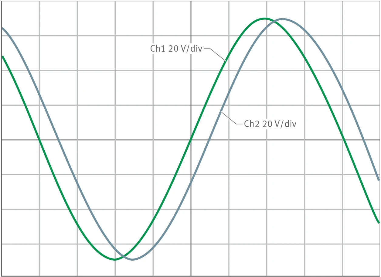
Figure 17: Phase offset 22.5° between the back EMFs. A two-channel oscilloscope shows the phase offset between two back EMF curves (Ch1 20 V/div, Ch2 20 V/div).
1.9.3 Evaluation of the temperature sensors
Incorrect or inaccurate alignment of the motors to each other may cause thermal overload of a motor. Integrated PTC sensors serve to protect the motor. The PTC sensors for each motor in the arrangement are connected in series and evaluated by a thermistor motor protection relay.
To prevent premature tripping of the motor protection system, Schaeffler Industrial Drives recommends using several or multi-channel thermistor motor protection relays in the event of three or more PTC monitoring circuits.
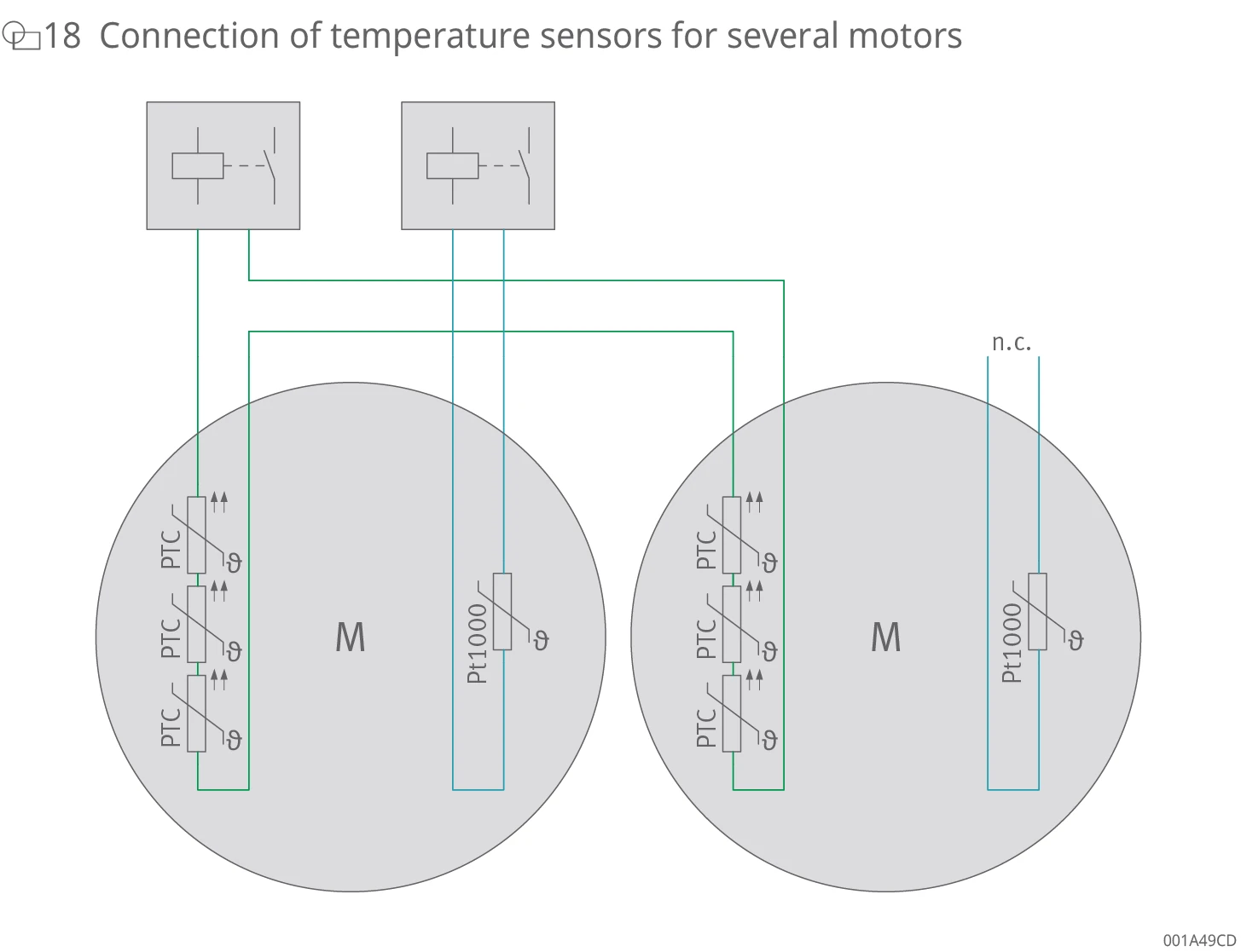
Figure 18: Connection of temperature sensors for several motors. The PTC (in series) of two motors M are connected to motor protection relays, with each motor also having a Pt1000 sensor (one marked n.c., not connected).
1.9.4 Resulting motor data
The parallel connection of structurally identical, individual motors results in new electrical data for the converter on the current replacement motor. These electrical data can easily be determined from the following data for the individual motors:
- The number of pole pairs, torque constant, voltage constant, time constant and speeds remain unchanged.
- Currents, torques and damping constant multiply with the number of individual motors.
- Resistance and inductance are divided by the number of individual motors.
1.10 Selection of direct drives for rotary applications
1.10.1 Cycle applications
Cyclic operation consists of successive positioning movements with movement breaks in between. A simple positioning action takes the form of a positively accelerated movement and subsequent braking. If the value for negative acceleration is the same, then the acceleration time and braking time are the same. The maximum angular velocity ωmax is reached at the end of an acceleration phase.
A cycle is described in the ω-t diagram. The ω-t diagram for cyclic operation shows a forward/backward rotation with breaks.
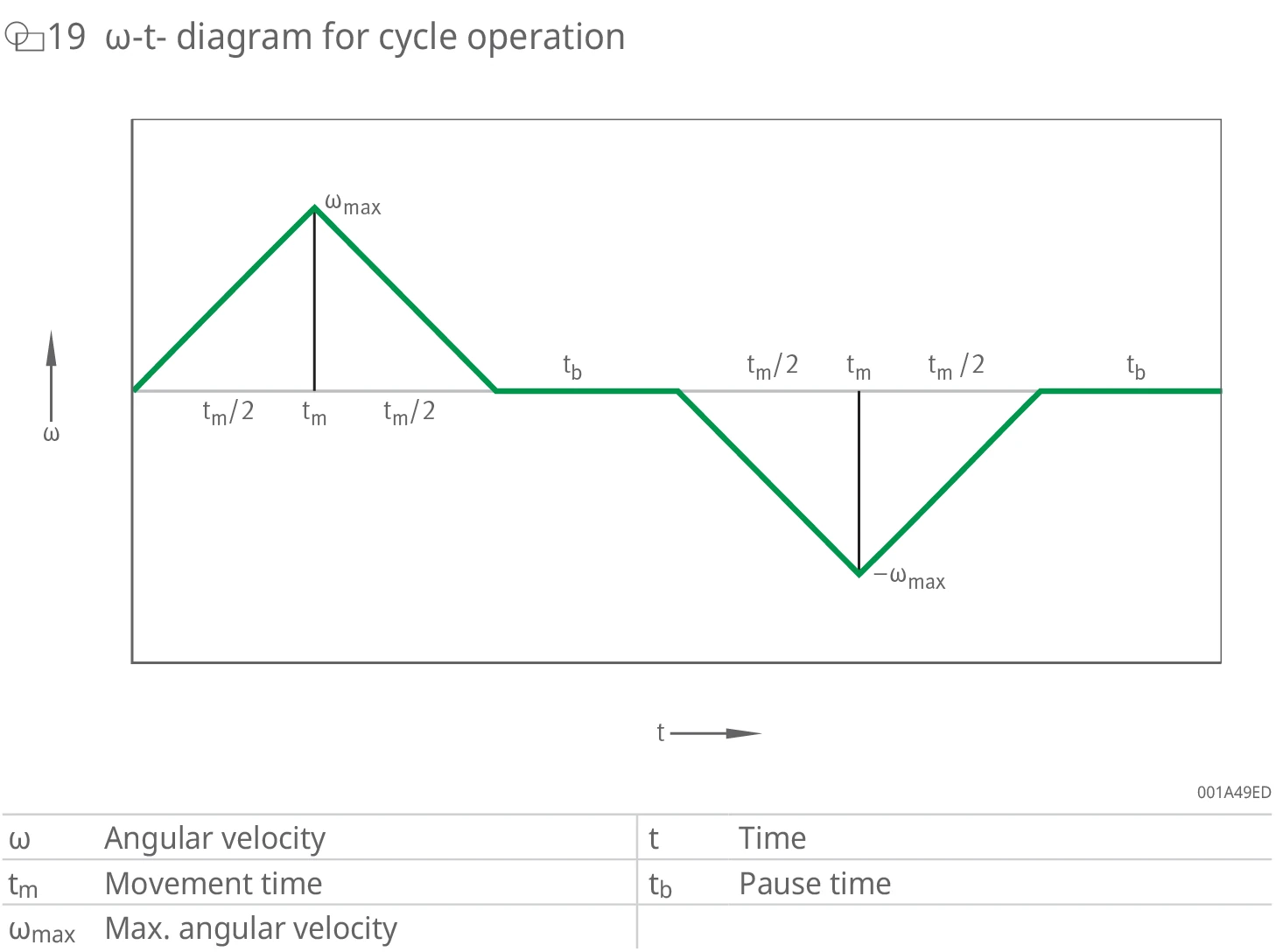
Figure 19: ω-t diagram for cycle operation. The vertical axis is angular velocity ω, the horizontal axis is time t. It shows forward/backward rotation with breaks, marking movement time tm, pause time tb and maximum angular velocity ωmax. Symbol definitions: ω=angular velocity, tm=movement time, ωmax=max. angular velocity, t=time, tb=pause time.
The α-t diagram for cyclic operation and the curve of the torque required for the movement are obtained from the forward/backward rotation with breaks:
Formula 6: Torque
T = J · α
| Symbol | Unit | Description |
|---|---|---|
| T | Nm | Torque |
| J | kg·m² | Mass moment of inertia |
| α | rad/s² | Angular acceleration |
Motor selection takes place on the basis of the following three criteria in accordance with the torque profile for a required cycle:
- max. torque in cycle ≤ Tp according to the performance data
- effective torque in cycle ≤ Tc (motor not cooled) or Tcw (water cooling) according to the performance data
- max. speed in cycle ≤ nlp according to the performance data
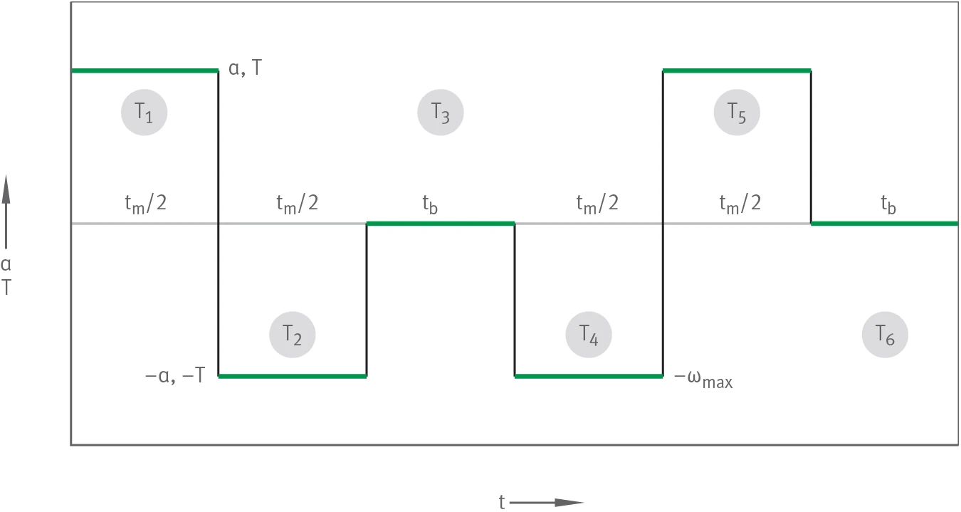
Figure 20: α-t diagram for cyclic operation. The vertical axis is angular acceleration α and torque T, the horizontal axis is time t. It shows six torque steps T1–T6. Symbol definitions: α=angular acceleration, tm=movement time, ωmax=max. angular velocity, t=time, tb=break time, T=torque, T1=torque step 1 (T1=T), T2=torque step 2 (T2=−T), T3=torque step 3 (T3=0), T4=torque step 4 (T4=−T), T5=torque step 5 (T5=T), T6=torque step 6 (T6=0).
The effective torque is equal to the root mean square of the torque profile consisting of six torque steps in the cycle.
Formula 7: Effective torque
Teff = √(T12·t1 + T22·t2 + … + T62·t6) / (t1 + t2 + … + t6)
| Symbol | Unit | Description |
|---|---|---|
| Teff | Nm | Effective torque |
| T1 | Nm | Torque step 1, T1 = T |
| t1 | s | Movement time 1, t1 = tm/2 |
| T2 | Nm | Torque step 2, T2 = −T |
| t2 | s | Movement time 2, t2 = tm/2 |
| T6 | Nm | Torque step 6, T6 = 0 |
| t6 | s | Movement time 6, t6 = tb |
We recommend a safety factor of 1.4 for the torques. The safety factor takes into account conditions such as motor operation in the non-linear range of the torque–current characteristic curve, for which the calculation equation for Teff only applies in approximate terms.
The effective torque can be calculated with the following torques:
- T1 = T
- T2 = −T
- T3 = 0
- T4 = −T
- T5 = T
- T6 = 0
The effective torque can be calculated with the following times:
- t1 = tm/2
- t2 = tm/2
- t3 = tb
- t4 = tm/2
- t5 = tm/2
- t6 = tb
Formula 8: Effective torque
Teff = T · √tm / (tm + tb)
Formula 9: Effective torque
Teff = J · α · √tm / (tm + tb)
If only torques of the same magnitude take effect in the cycle, this equation applies to the effective torque (Formula 9). Mass moment of inertia and angular accelerations are constant. The movement time divided by the sum of the movement time and break time goes underneath the root. The cycle time is included in the denominator.
Angular acceleration, max. angular velocity and max. rotational speed of a positioning movement can be calculated with the following:
Formula 10: Angular acceleration
α = (4 · φ) / tm2
| Symbol | Unit | Description |
|---|---|---|
| α | rad/s² | Angular acceleration |
| φ | ° | Movement angle |
| tm | s | Movement time |
Formula 11: Max. angular velocity
ωmax = (2 · φ) / tm
| Symbol | Unit | Description |
|---|---|---|
| tm | s | Movement time |
Formula 12: Max. speed
nmax = (30 / π) · ωmax
The calculation method shown here is idealised and simplified. For example, the increase in angular acceleration is infinitely high. In practice, angular acceleration is limited by motor inductance or other components. Safety factors or, in the case of highly dynamic movements, additional times of 15 ms to 20 ms per positioning operation are used to account for these effects in the design.
1.10.2 Example of cycle applications
Table 10: Specified values
| Specified values | Unit | Value |
|---|---|---|
| Movement angle φ | ° | 180 |
| Movement time tm | s | 0,5 |
| Cycle time tm + tb | s | 1,35 |
| Mass moment of inertia J | kg·m² | 2,5 |
| Frictional torque TF | Nm | 8 |
| Safety factor SF | – | 1,4 |
Calculation
Movement angle conversion:
Formula 13: Movement angle conversion
φ = (π / 180) · 180 rad = 3,142 rad
Max. angular velocity:
Formula 14: Max. angular velocity
ωmax = (2 · φ) / tm = (2 · 3,142) / 0,5 rad/s = 12,57 rad/s
Max. speed:
Formula 15: Max. speed
nmax = (30 / π) · ωmax = (30 / π) · 12,57 1/s = 120 min⁻¹
Angular acceleration:
Formula 16: Angular acceleration
α = (4 · φ) / tm2 = (4 · 3,142) / 0,52 rad/s² = 50,27 rad/s²
Taking into account the bearing frictional torque TF, the maximum torque is obtained as follows:
Formula 17: Max. torque
Tmax = (J · α) + TF = (2,5 · 50,27) + 8 = 133,68 Nm
Effective torque, taking into account the bearing frictional torque TF:
Formula 18: Effective torque, taking into account the bearing frictional torque
Teff = ( J · α · √tm / (tm + tb) ) + TF = ( 2,5 · 50,27 · √0,5 / 1,35 ) + 8 = 84,48 Nm
Taking into account the safety factor SF, the motor is selected according to the following requirements:
Tsafe max = Tmax × 1,4 ≤ TP
Tsafe eff = Teff × 1,4 ≤ Tcw
nmax ≤ nlp
A safety factor for speed is only required when using frequency inverters with an unstabilised DC link voltage. In the present case, a frequency inverter with a stabilised DC link voltage of UDCL = 600 V is used. It is therefore permissible to work without a safety factor for speed, and nmax ≤ nlp applies. If nmax > nlp, the operating point Tsafe max at nmax can be verified using the torque–speed characteristic curve at the corresponding DC link voltage.
The calculation results in the following motor requirements:
Without safety factor:
- Tp = 133,68 Nm
- Tcw = 84,48 Nm
With safety factor:
- Tsafe max = 187,15 Nm
- Tsafe eff = 118,27 Nm
Motor RIB17-3P-168x50-Z0.7 (Tp = 233 Nm, Tcw = 123 Nm, nlp = 150 min⁻¹) meets the requirement in the sample calculation in full.
1.10.3 NC rotary table applications
For water-cooled rotary table applications, the speed n, moment of inertia J, processing torque in motion TW and stall torque Tsw as well as the angular accelerations α in S1 operation and αmax in S6 operation are usually known. Although the effective times of the torques change on a frequent basis, determining the effective torque as a continuous torque and the maximum torque as accurately as possible is necessary in order to select the optimal motor and to prevent exceeding of the maximum permissible winding temperature.
All load torques occurring during motor operation are incorporated into the torque calculation.
1.10.4 Example of NC rotary table applications
Table 11: Specified values
| Specified values | Unit | Value |
|---|---|---|
| Speed n | min⁻¹ | 60 |
| Mass moment of inertia J | kg·m² | 4 |
| Processing torque TW | Nm | 300 |
| Frictional torque TF | Nm | 50 |
| Weight force (additional torque) TZ | Nm | 0 |
| Angular acceleration in S1 mode αS1 | °/s² | 9000 |
| Max. angular acceleration in S6 operation for 3 s αmax | °/s² | 20000 |
| Safety factor SF | – | 1,4 |
Calculation
Conversion of angular acceleration into rad/s²:
Formula 19: Angular acceleration
αS1 = (π / 180) · αS1 [°/s²] = (π / 180) · 9000 = 157 rad/s²
Formula 20: Max. angular acceleration
αmax = (π / 180) · αmax [°/s²] = (π / 180) · 20000 = 349 rad/s²
Motor selection is based on the cooled stall torque Tsw and on the torques in motion for S1 operation, Tcw, and S6 operation, Tp. The safety factor SF of 1.4 ensures that the position can be reliably maintained and the control system safely responds to deviations.
Formula 21: Cooled stall torque, with water cooling
Tsw = ( TW + TF + TZ ) · 1,4 = 490 N
| Symbol | Unit | Description |
|---|---|---|
| Tsw | Nm | Stall torque, cooled |
| TW | Nm | Processing torque |
| TF | Nm | Bearing frictional torque |
| TZ | Nm | Weight force (additional torque) |
Formula 22: Cooled continuous torque, with water cooling
Tcw = ( J · αS1 + TW + TF + TZ ) · 1,4 = 1369 N
| Symbol | Unit | Description |
|---|---|---|
| Tcw | Nm | Continuous torque, cooled |
| J | kg·m² | Mass moment of inertia |
| αS1 | rad/s² | Angular acceleration in S1 operation |
| TW | Nm | Processing torque |
| TF | Nm | Bearing frictional torque |
| TZ | Nm | Weight force (additional torque) |
Formula 23: Peak torque
Tp = ( J · αmax + TW + TF + TZ ) · 1,4 = 2444 N
| Symbol | Unit | Description |
|---|---|---|
| Tp | Nm | Peak torque |
| J | kg·m² | Mass moment of inertia |
| αmax | rad/s² | Max. angular acceleration |
| TW | Nm | Processing torque |
| TF | Nm | Bearing frictional torque |
| TZ | Nm | Weight force (additional torque) |
The calculation results in the following requirements:
- Tp = 2444 Nm
- Tcw = 1369 Nm
Motor RIB13-3P-690×50-Z4.2 (Tp = 3627 Nm, Tcw = 2166 Nm, nlp = 61 min⁻¹) meets the requirements in the sample calculation in full.
Speed control is used in this example. The NC rotary table should first start at a defined speed. The NC rotary table then processes the workpiece at this speed.
If a positioning operation is additionally required, as in the case of so-called reversers in position control, the required speed at TP must be increased by a safety factor of 10 % to 20 %. The limiting speed nlp of the motor must then be greater than the calculated speed complete with additional value.
Note: The values, formulas and examples listed in this chapter are all taken from the technical principles chapter of the Schaeffler RE 1 catalogue. Binding data is provided in the quotation and delivery drawing. Subject to change without notice.